Tags: algorithm chemistry variational
This tutorial demonstrates how to implement the Variational Quantum Eigensolver (VQE) algorithm to find the ground state energy of the hydrogen molecule (H₂). We use OpenFermion for generating molecular Hamiltonians.
The workflow is as follows:
Convert the molecular Hamiltonian to qubit operators
Create a parametrized quantum circuit (ansatz)
Implement VQE optimization
Analyze the energy landscape across different atomic distances
We show how to solve quantum chemistry problems using quantum computing, focusing on finding the minimum-energy structure of the H₂ molecule.
# Required packages can be installed with the following command
# !pip install openfermion pyscf openfermionpyscf
import os
import warnings
import matplotlib.pyplot as plt
import numpy as np
import openfermion.chem as of_chem
import openfermion.transforms as of_trans
import openfermionpyscf as of_pyscf
from qiskit_aer.primitives import EstimatorV2
from scipy.optimize import minimize
import qamomile.circuit as qmc
import qamomile.observable as qm_o
from qamomile.circuit.algorithm.basic import cx_entangling_layer, ry_layer, rz_layer
from qamomile.qiskit import QiskitTranspiler
from qamomile.qiskit.transpiler import QiskitExecutor
docs_test_mode = os.environ.get("QAMOMILE_DOCS_TEST") == "1"Creating the Hamiltonian of the Hydrogen Molecule
basis = "sto-3g"
multiplicity = 1
charge = 0
distance = 0.977
geometry = [["H", [0, 0, 0]], ["H", [0, 0, distance]]]
description = "tmp"
molecule = of_chem.MolecularData(geometry, basis, multiplicity, charge, description)
molecule = of_pyscf.run_pyscf(molecule, run_scf=True, run_fci=True)
n_qubit = molecule.n_qubits
n_electron = molecule.n_electrons
# H2 in the STO-3G basis has 2 spatial orbitals -> 4 spin orbitals -> 4 qubits,
# and is a 2-electron molecule.
assert n_qubit == 4
assert n_electron == 2
fermionic_hamiltonian = of_trans.get_fermion_operator(
    molecule.get_molecular_hamiltonian()
)
jw_hamiltonian = of_trans.jordan_wigner(fermionic_hamiltonian)
Converting to a Qamomile Hamiltonian
In this section, we convert the OpenFermion Hamiltonian to the Qamomile format. After applying the Jordan–Wigner transformation to convert fermionic operators to qubit operators, we use custom conversion functions to create a Hamiltonian representation compatible with Qamomile.
def operator_to_qamomile(operators: tuple[tuple[int, str], ...]) -> qm_o.Hamiltonian:
    pauli = {"X": qm_o.X, "Y": qm_o.Y, "Z": qm_o.Z}
    H = qm_o.Hamiltonian()
    H.constant = 1.0
    for ope in operators:
        H *= pauli[ope[1]](ope[0])
    return H


def openfermion_to_qamomile(of_h) -> qm_o.Hamiltonian:
    H = qm_o.Hamiltonian()
    for k, v in of_h.terms.items():
        if len(k) == 0:
            H.constant += v
        else:
            H += operator_to_qamomile(k) * v
    return H


hamiltonian = openfermion_to_qamomile(jw_hamiltonian)
assert hamiltonian.num_qubits == n_qubit
Creating the VQE Ansatz
In this section, we create a Hardware Efficient SU(2) ansatz for the VQE algorithm using the @qkernel decorator. An ansatz is a parametrized quantum circuit that prepares a trial wavefunction. We build it by combining ry_layer, rz_layer, and a linear CX entangling layer, and finally compute the expectation value of the Hamiltonian using expval.
@qmc.qkernel
def vqe_ansatz(
    n: qmc.UInt,
    reps: qmc.UInt,
    thetas: qmc.Vector[qmc.Float],
    H: qmc.Observable,
) -> qmc.Float:
    q = qmc.qubit_array(n, name="q")
    for r in qmc.range(reps):
        base = r * 2 * n
        q = ry_layer(q, thetas, base)
        q = rz_layer(q, thetas, base + n)
        q = cx_entangling_layer(q)
    # Final rotation layer
    final_base = reps * 2 * n
    q = ry_layer(q, thetas, final_base)
    q = rz_layer(q, thetas, final_base + n)
    return qmc.expval(q, H)
Running VQE with Qiskit
In this section, we transpile the VQE kernel to an executable object using QiskitTranspiler. The default executor runs this object and returns the expectation value, which the defined qkernel computes using expval. Thus, the user only needs to implement the optimisation loop.
transpiler = QiskitTranspiler()
reps = 4

executable = transpiler.transpile(
    vqe_ansatz,
    bindings={"n": n_qubit, "reps": reps, "H": hamiltonian},
    parameters=["thetas"],
)

# Transpiled quantum circuit
executable.quantum_circuit.draw("mpl")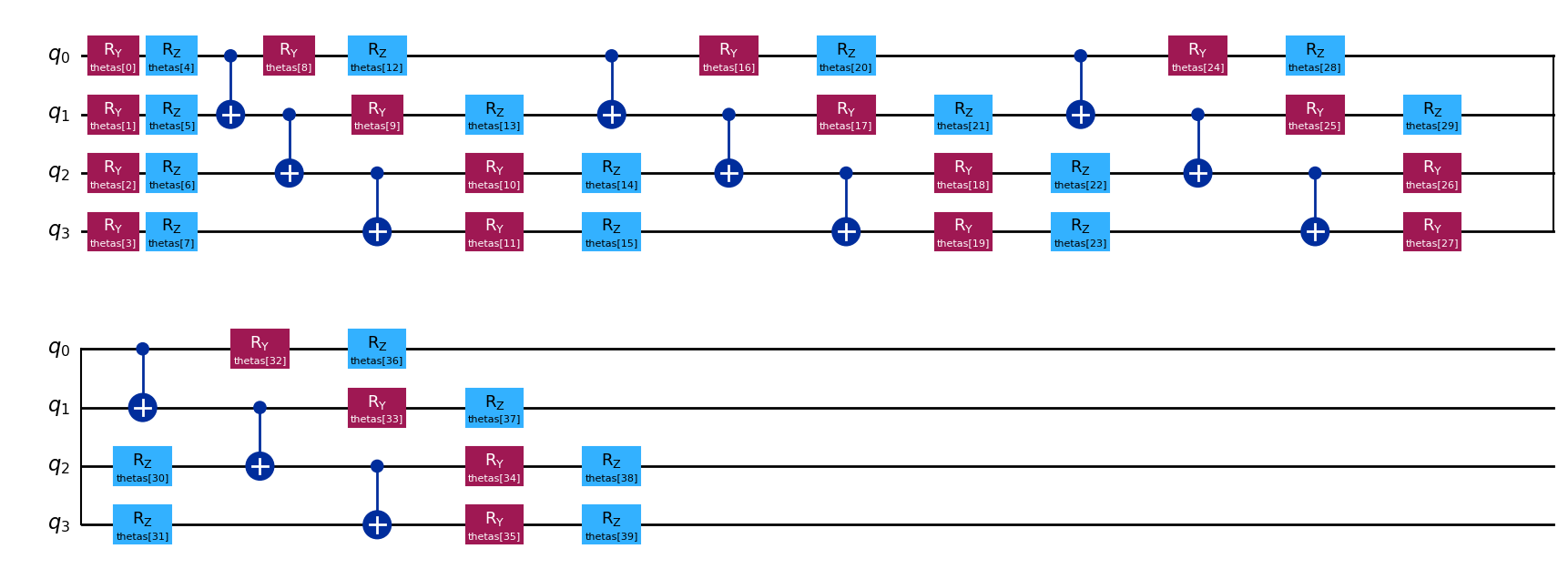
cost_history = []
executor = QiskitExecutor(estimator=EstimatorV2())


def cost_fn(param_values):
    job = executable.run(executor, bindings={"thetas": list(param_values)})
    return job.result()


def cost_callback(param_values):
    cost_history.append(cost_fn(param_values))


num_params = len(executable.parameter_names)
rng = np.random.default_rng(42)
initial_params = rng.uniform(0, np.pi, num_params)
# Each rep emits one RY layer (n parameters) and one RZ layer (n parameters);
# the final pre-CX layer adds one more RY + RZ pair. So the parameter count is
# (reps + 1) * 2 * n_qubit.
assert num_params == (reps + 1) * 2 * n_qubit
assert initial_params.shape == (num_params,)

# Run VQE optimization
maxiter = 1 if docs_test_mode else 50
warnings.filterwarnings("ignore", message="Maximum number of iterations")
result = minimize(
    cost_fn,
    initial_params,
    method="BFGS",
    options={"disp": True, "maxiter": maxiter, "gtol": 1e-6},
    callback=cost_callback,
)
print(result)
# Variational principle: any trial energy is an upper bound on the FCI
# ground-state energy, regardless of how short the BFGS budget is.
# ``run_fci=True`` was passed to ``of_pyscf.run_pyscf`` above, so
# ``molecule.fci_energy`` is populated; openfermion's stub declares it
# ``float | None`` to cover the ``run_fci=False`` case, so narrow here.
fci_ref = molecule.fci_energy
assert fci_ref is not None
assert result.fun >= fci_ref - 1e-9
assert len(result.x) == num_params
Current function value: -1.105860
Iterations: 50
Function evaluations: 2091
Gradient evaluations: 51
message: Maximum number of iterations has been exceeded.
success: False
status: 1
fun: -1.105859672342776
x: [ 3.123e+00 1.022e+00 ... 1.306e+00 2.499e+00]
nit: 50
jac: [-2.432e-04 7.428e-05 ... -2.052e-04 -1.994e-04]
hess_inv: [[ 3.779e+00 5.352e-01 ... 5.601e-01 4.337e-01]
[ 5.352e-01 1.988e+00 ... -7.801e-01 -2.818e-01]
...
[ 5.601e-01 -7.801e-01 ... 3.531e+00 2.205e+00]
[ 4.337e-01 -2.818e-01 ... 2.205e+00 3.404e+00]]
nfev: 2091
njev: 51
plt.plot(cost_history)
plt.plot(
    range(len(cost_history)),
    [fci_ref] * len(cost_history),
    linestyle="dashed",
    color="black",
    label="Exact Solution",
)
plt.legend()
plt.show()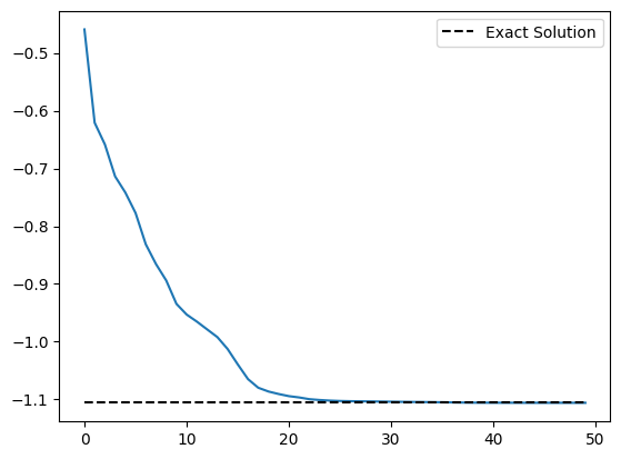
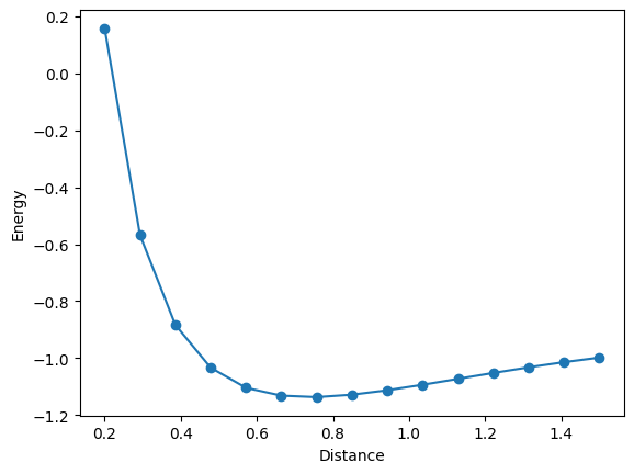
Changing the Distance Between Atoms
def hydrogen_molecule(bond_length):
    basis = "sto-3g"
    multiplicity = 1
    charge = 0
    geometry = [["H", [0, 0, 0]], ["H", [0, 0, bond_length]]]
    description = "tmp"
    molecule = of_chem.MolecularData(geometry, basis, multiplicity, charge, description)
    molecule = of_pyscf.run_pyscf(molecule, run_scf=True, run_fci=True)
    fermionic_hamiltonian = of_trans.get_fermion_operator(
        molecule.get_molecular_hamiltonian()
    )
    jw_hamiltonian = of_trans.jordan_wigner(fermionic_hamiltonian)
    return openfermion_to_qamomile(jw_hamiltonian), molecule.fci_energy


n_points = 3 if docs_test_mode else 15
bond_lengths = np.linspace(0.2, 1.5, n_points)
assert bond_lengths.shape == (n_points,)
energies = []
for bond_length in bond_lengths:
    hamiltonian, fci_energy = hydrogen_molecule(bond_length)
    # H2 remains a 4-qubit problem regardless of bond length.
    assert hamiltonian.num_qubits == 4

    executable = transpiler.transpile(
        vqe_ansatz,
        bindings={"n": hamiltonian.num_qubits, "reps": reps, "H": hamiltonian},
        parameters=["thetas"],
    )

    num_params = len(executable.parameter_names)
    initial_params = rng.uniform(0, np.pi, num_params)
    result = minimize(
        cost_fn,
        initial_params,
        method="BFGS",
        options={"maxiter": maxiter, "gtol": 1e-6},
    )

    energies.append(result.fun)
    # ``run_fci=True`` was passed, so ``fci_energy`` is populated;
    # narrow off openfermion's ``float | None`` stub.
    assert fci_energy is not None
    # Variational principle holds at every bond length.
    assert result.fun >= fci_energy - 1e-9

    print("distance: ", bond_length, "energy: ", result.fun, "fci_energy: ", fci_energy)

assert len(energies) == n_points
distance: 0.2 energy: 0.15749329365461995 fci_energy: 0.15748213479836526
distance: 0.29285714285714287 energy: -0.5679193889010842 fci_energy: -0.5679447209710013
distance: 0.38571428571428573 energy: -0.8833483653566578 fci_energy: -0.8833596636183383
distance: 0.4785714285714286 energy: -1.033582342419856 fci_energy: -1.0336011797110967
distance: 0.5714285714285714 energy: -1.1041774579732506 fci_energy: -1.1042094222435166
distance: 0.6642857142857144 energy: -1.1316536828860908 fci_energy: -1.1323508827075506
distance: 0.7571428571428571 energy: -1.136896895687888 fci_energy: -1.1369026717971333
distance: 0.8500000000000001 energy: -1.128359326275411 fci_energy: -1.128361878458112
distance: 0.9428571428571428 energy: -1.1127239395799284 fci_energy: -1.1127252078468768
distance: 1.0357142857142858 energy: -1.093476087896891 fci_energy: -1.093476088229404
distance: 1.1285714285714286 energy: -1.0727482357543656 fci_energy: -1.0727578805453502
distance: 1.2214285714285713 energy: -1.0520071096366461 fci_energy: -1.052008162170845
distance: 1.3142857142857143 energy: -1.0322163897827572 fci_energy: -1.0322400306247084
distance: 1.4071428571428573 energy: -1.014138609349133 fci_energy: -1.0141470586695496
distance: 1.5 energy: -0.998088727242389 fci_energy: -0.9981493534714101
plt.plot(bond_lengths, energies, "-o")
plt.xlabel("Distance")
plt.ylabel("Energy")
plt.show()