QAOA for Graph Partitioning - Qamomile Documentation

This tutorial demonstrates how to solve the graph partitioning problem using the Quantum Approximate Optimization Algorithm (QAOA) with Qamomile.

The workflow is:

JijModeling problem → problem.eval() → QAOAConverter → transpile → sample → decode

Formulate the problem with JijModeling.
Create an instance with concrete data.
Use QAOAConverter to build the QAOA circuit and Hamiltonian.
Optimize the variational parameters with a classical optimizer.
Sample the optimized circuit and decode the results.

# Install the latest Qamomile through pip!
# !pip install qamomile

Problem Formulation¶

Given an undirected graph $G = (V, E)$ , the goal is to partition the vertices into two groups of equal size while minimizing the number of edges between the two groups.

Objective:

\min \sum_{(u,v) \in E} \bigl[x_u(1 - x_v) + x_v(1 - x_u)\bigr]

(1)

Constraint:

\sum_{u \in V} x_u = \frac{|V|}{2}

(2)

where $x_u \in \{0, 1\}$ indicates which partition vertex $u$ belongs to.

Define the Problem with JijModeling¶

import jijmodeling as jm

problem = jm.Problem("Graph Partitioning")


@problem.update
def _(problem: jm.DecoratedProblem):
    V = problem.Dim()
    E = problem.Natural(ndim=2)  # edge list: [[u1,v1], [u2,v2], ...]
    x = problem.BinaryVar(shape=(V,))

    # Objective: minimize edges cut between partitions
    problem += (
        E.rows().map(lambda e: x[e[0]] * (1 - x[e[1]]) + x[e[1]] * (1 - x[e[0]])).sum()
    )

    # Constraint: equal partition sizes
    problem += problem.Constraint("equal_partition", x.sum() == V / 2)


problem

Graph Instance¶

We use a fixed 8-node graph with 16 edges for reproducibility.

import matplotlib.pyplot as plt
import networkx as nx

num_nodes = 8
edge_list = [
    [0, 2],
    [0, 3],
    [0, 4],
    [1, 2],
    [1, 3],
    [1, 4],
    [1, 5],
    [1, 7],
    [2, 3],
    [2, 6],
    [3, 5],
    [4, 5],
    [4, 6],
    [5, 6],
    [5, 7],
    [6, 7],
]

G = nx.Graph()
G.add_nodes_from(range(num_nodes))
G.add_edges_from(edge_list)

pos = nx.spring_layout(G, seed=1)
plt.figure(figsize=(5, 5))
nx.draw(
    G,
    pos,
    with_labels=True,
    node_color="white",
    node_size=700,
    edgecolors="black",
)
plt.title(f"Graph: {G.number_of_nodes()} nodes, {G.number_of_edges()} edges")
plt.show()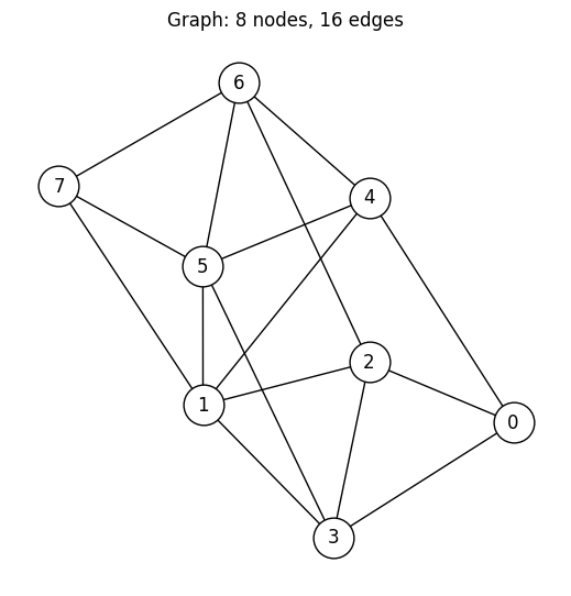

Create the Instance¶

We extract the edge list from the graph and evaluate the JijModeling problem with the concrete data.

instance_data = {"V": num_nodes, "E": edge_list}
instance = problem.eval(instance_data)

Set Up the QAOAConverter¶

QAOAConverter takes an OMMX instance and internally:

Converts the problem to a QUBO (Quadratic Unconstrained Binary Optimization) form.
Transforms from BINARY variables to SPIN variables.
Builds the cost Hamiltonian as a sum of Pauli-Z operators.

Because the original problem has a constraint, the QUBO formulation folds it into the objective as a penalty term. This means the energy values from the decoded samples are not the original objective (number of cut edges) — they include the penalty. We will need to check feasibility and compute the true objective separately.

from qamomile.optimization.qaoa import QAOAConverter

converter = QAOAConverter(instance)
converter.spin_model = converter.spin_model.normalize_by_abs_max()
hamiltonian = converter.get_cost_hamiltonian()
print(hamiltonian)

Hamiltonian((Z0, Z1): 1.0, (Z0, Z5): 1.0, (Z0, Z6): 1.0, (Z0, Z7): 1.0, (Z1, Z6): 1.0, (Z2, Z4): 1.0, (Z2, Z5): 1.0, (Z2, Z7): 1.0, (Z3, Z4): 1.0, (Z3, Z6): 1.0, (Z3, Z7): 1.0, (Z4, Z7): 1.0)

Transpile to an Executable Circuit¶

converter.transpile() builds a QAOA ansatz circuit with p layers and compiles it into an ExecutableProgram. The variational parameters gammas (cost layer) and betas (mixer layer) remain as runtime parameters.

from qamomile.qiskit import QiskitTranspiler

transpiler = QiskitTranspiler()
p = 5  # number of QAOA layers
executable = converter.transpile(transpiler, p=p)

Optimize the QAOA Parameters¶

We use executable.sample() to evaluate the cost at each iteration of the classical optimizer. The optimizer explores different gammas and betas to minimize the mean energy of the sampled bitstrings.

import numpy as np
from qiskit_aer import AerSimulator
from scipy.optimize import minimize

executor = transpiler.executor(backend=AerSimulator(seed_simulator=900))

rng = np.random.default_rng(900)
initial_params = rng.uniform(0, np.pi, 2 * p)

cost_history = []


def cost_fn(params):
    gammas = list(params[:p])
    betas = list(params[p:])
    job = executable.sample(
        executor,
        shots=2048,
        bindings={"gammas": gammas, "betas": betas},
    )
    result = job.result()
    decoded = converter.decode(result)
    energy = decoded.energy_mean()
    cost_history.append(energy)
    return energy


res = minimize(
    cost_fn,
    initial_params,
    method="COBYLA",
    options={"maxiter": 1000},
)

print(f"Optimized cost: {res.fun:.3f}")
print(f"Optimal params: {[round(v, 4) for v in res.x]}")
print(f"Function evaluations: {res.nfev}")

Optimized cost: 14.144
Optimal params: [np.float64(0.4449), np.float64(1.1507), np.float64(2.8692), np.float64(0.5418), np.float64(2.5772), np.float64(1.0364), np.float64(3.6029), np.float64(0.1049), np.float64(3.0026), np.float64(0.7662)]
Function evaluations: 140

plt.figure(figsize=(8, 4))
plt.plot(cost_history, color="#2696EB")
plt.xlabel("Iteration")
plt.ylabel("Cost (mean energy)")
plt.title("QAOA Optimization Progress")
plt.show()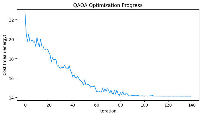

Sample with Optimized Parameters¶

With the optimized parameters, we sample the circuit to collect candidate solutions as bitstrings.

gammas_opt = list(res.x[:p])
betas_opt = list(res.x[p:])

sample_result = executable.sample(
    executor,
    shots=1000,
    bindings={"gammas": gammas_opt, "betas": betas_opt},
).result()

decoded = converter.decode(sample_result)

Analyze the Results¶

Feasibility Check¶

QAOA samples are candidate solutions — they are not guaranteed to satisfy the original constraints. The constraint $\sum x_u = |V|/2$ was folded into the QUBO as a penalty, so infeasible bitstrings can still appear in the output.

We must filter samples by feasibility before interpreting them as valid partitions.

def is_feasible(sample: dict[int, int]) -> bool:
    """Check if a sample satisfies the equal partition constraint."""
    return sum(sample.values()) == num_nodes // 2


def count_cut_edges(sample: dict[int, int], graph: nx.Graph) -> int:
    """Compute the true objective: number of edges between the two partitions."""
    cuts = 0
    for u, v in graph.edges():
        if sample.get(u, 0) != sample.get(v, 0):
            cuts += 1
    return cuts

feasible_results = []
for sample, energy, occ in zip(
    decoded.samples, decoded.energy, decoded.num_occurrences
):
    if is_feasible(sample):
        obj = count_cut_edges(sample, G)
        feasible_results.append((sample, obj, occ))

total_feasible = sum(occ for _, _, occ in feasible_results)
total_samples = sum(decoded.num_occurrences)

print(
    f"Feasible samples: {total_feasible} / {total_samples} "
    f"({100 * total_feasible / total_samples:.1f}%)"
)

Feasible samples: 587 / 1000 (58.7%)

Best Feasible Solution¶

Among the feasible samples, we select the one with the fewest cut edges (the true objective).

if feasible_results:
    feasible_results.sort(key=lambda x: x[1])
    best_sample, best_obj, best_count = feasible_results[0]
    print(f"Best feasible solution: {best_sample}")
    print(f"Cut edges:             {best_obj}")
    print(f"Occurrences:           {best_count}")
else:
    print("No feasible solution found. Try increasing p or maxiter.")
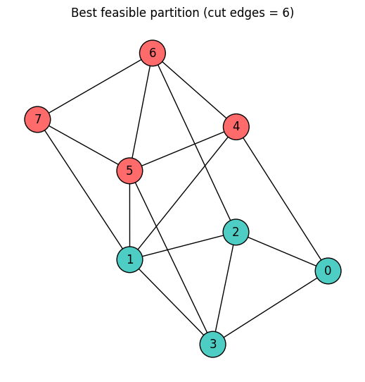
    best_sample = None

Best feasible solution: {0: 0, 1: 0, 2: 0, 3: 0, 4: 1, 5: 1, 6: 1, 7: 1}
Cut edges:             6
Occurrences:           131

Objective Value Distribution¶

We plot the distribution of the true objective value (cut edges) for feasible samples only.

from collections import Counter

if feasible_results:
    obj_counts = Counter()
    for _, obj, occ in feasible_results:
        obj_counts[obj] += occ

    objs = sorted(obj_counts.keys())
    counts = [obj_counts[o] for o in objs]

    plt.figure(figsize=(8, 4))
    plt.bar([str(o) for o in objs], counts, color="#2696EB")
    plt.xlabel("Cut edges (objective value)")
    plt.ylabel("Frequency")
    plt.title("Distribution of Feasible Solutions")
    plt.show()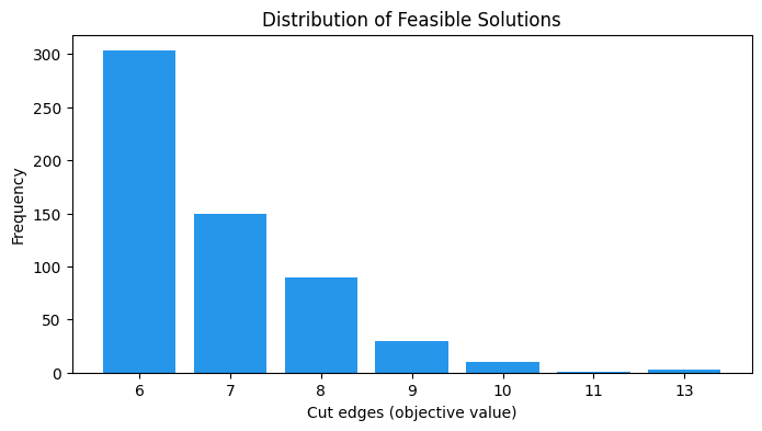

Visualize the Best Partition¶

We color the graph nodes according to the best feasible partition found by QAOA.

if best_sample is not None:
    color_map = [
        "#FF6B6B" if best_sample.get(i, 0) == 1 else "#4ECDC4" for i in range(num_nodes)
    ]

    plt.figure(figsize=(5, 5))
    nx.draw(
        G,
        pos,
        with_labels=True,
        node_color=color_map,
        node_size=700,
        edgecolors="black",
    )
    plt.title(f"Best feasible partition (cut edges = {best_obj})")
    plt.show()