Hamiltonian Simulation with Suzuki–Trotter (Rabi oscillation)

Tags: algorithm primitive simulation

Simulating the time evolution $e^{-iHt}$ of a quantum system is one of the canonical applications of a quantum computer. When the Hamiltonian splits into non-commuting pieces $H = A + B$ with $[A, B] \neq 0$ , the naive factorisation $e^{-i(A+B)t} = e^{-iAt}\,e^{-iBt}$ is wrong; the standard fix is Trotter–Suzuki product formulas, which interleave short evolutions of each piece. The error decreases as we take smaller steps (Lie–Trotter, first order), symmetrise the step (Strang, second order), or nest the symmetric step recursively via Suzuki’s construction (any even order).

This article builds these approximations end-to-end in Qamomile on a one-qubit Rabi Hamiltonian so the Trotter error is measurable. We start with $S_1$ and $S_2$ , then write the full Suzuki fractal recursion as a self-recursive @qkernel that takes the target order as a UInt parameter — the transpiler resolves the recursion by iterating inline + partial-evaluation under a concrete order binding, so the emitted circuit is flat regardless of how deep the recursion went. Finally, we verify the textbook convergence rates ( $S_k$ ’s fidelity error scales as $\Delta t^{2k}$ ) against the exact 2x2 propagator.

# Install the latest Qamomile through pip!
# !pip install qamomile

import matplotlib.pyplot as plt
import numpy as np
from qiskit import QuantumCircuit, transpile as qk_transpile
from qiskit_aer import AerSimulator
from scipy.linalg import expm

import qamomile.circuit as qmc
import qamomile.observable as qm_o
from qamomile.circuit.algorithm import trotterized_time_evolution
from qamomile.qiskit import QiskitTranspiler

The Rabi Hamiltonian¶

A single two-level system driven on resonance is governed by

H = \underbrace{\tfrac{\omega}{2} Z}_{H_z} + \underbrace{\tfrac{\Omega}{2} X}_{H_x}.

(1)

Because $[Z, X] \neq 0$ , splitting $H$ into $H_z$ and $H_x$ introduces a Trotter error that is easy to see even on a single qubit. Starting from $|0\rangle$ , the excitation probability oscillates as $P_{|1\rangle}(t) = (\Omega/E)^2 \sin^2(Et/2)$ with $E = \sqrt{\omega^2 + \Omega^2}$ .

In Qamomile we build $H_z$ and $H_x$ as two separate Observables and pack them into a Python list. A @qkernel declares that list as Vector[Observable]; binding the list at transpile time expands any iteration over Hs.shape[0] into per-term pauli_evolve calls.

omega = 1.2
Omega = 0.8
T = 1.5

Hz = 0.5 * omega * qm_o.Z(0)
Hx = 0.5 * Omega * qm_o.X(0)
Hs = [Hz, Hx]

Exact reference state¶

A 2x2 matrix exponential gives the exact state $|\psi(T)\rangle = e^{-iHT}|0\rangle$ , which each Trotter approximation is judged against via the fidelity error $1 - |\langle\psi_\text{exact}|\psi_\text{trotter}\rangle|$ .

X_mat = np.array([[0, 1], [1, 0]], dtype=complex)
Z_mat = np.array([[1, 0], [0, -1]], dtype=complex)
H_mat = 0.5 * omega * Z_mat + 0.5 * Omega * X_mat
sv_exact = expm(-1j * T * H_mat) @ np.array([1.0, 0.0], dtype=complex)

def statevector(circuit) -> np.ndarray:
    """Strip measurements, lower PauliEvolutionGate, and read out the state.

    The default ``pauli_evolve`` emitter produces a ``PauliEvolutionGate``, which
    is not in AerSimulator's native basis.  We run a shallow Qiskit transpile
    pass to expand it into elementary rotations before simulating.
    """
    stripped = QuantumCircuit(*circuit.qregs)
    for instr in circuit.data:
        if instr.operation.name not in ("measure", "save_statevector"):
            stripped.append(instr)
    stripped = qk_transpile(
        stripped,
        basis_gates=["u", "cx", "rx", "ry", "rz", "h", "p", "sx", "x", "y", "z"],
    )
    stripped.save_statevector()
    sim = AerSimulator(method="statevector")
    return np.asarray(sim.run(stripped).result().get_statevector())

$S_1$ : First-order Suzuki–Trotter decomposition (Lie–Trotter)¶

The simplest split is

S_1(\Delta t) = e^{-i H_x \Delta t}\, e^{-i H_z \Delta t},

(2)

applied $N$ times for a total evolution time $T = N \Delta t$ . Per step the local error is $O(\Delta t^2)$ ; integrated over $N = T/\Delta t$ steps the global state-norm error is $O(\Delta t)$ .

We write one step as a small helper @qkernel: the qubit register is threaded through, evolved under $H_z$ and then $H_x$ . The outer kernel rabi_s1 repeats that step $N$ times, where n_steps is a UInt parameter so the same kernel transpiles for any $N$ at bind-time.

@qmc.qkernel
def s1_step(
    q: qmc.Vector[qmc.Qubit], Hs: qmc.Vector[qmc.Observable], dt: qmc.Float
) -> qmc.Vector[qmc.Qubit]:
    q = qmc.pauli_evolve(q, Hs[0], dt)
    q = qmc.pauli_evolve(q, Hs[1], dt)
    return q

@qmc.qkernel
def rabi_s1(
    Hs: qmc.Vector[qmc.Observable], dt: qmc.Float, n_steps: qmc.UInt
) -> qmc.Vector[qmc.Bit]:
    q = qmc.qubit_array(1, "q")
    for _ in qmc.range(n_steps):
        q = s1_step(q, Hs, dt)
    return qmc.measure(q)

$S_2$ : Second-order Suzuki–Trotter decomposition (Strang splitting)¶

Symmetrising the step around the middle term cancels the leading error:

S_2(\Delta t) = e^{-i H_z \Delta t/2}\, e^{-i H_x \Delta t}\, e^{-i H_z \Delta t/2}.

(3)

The local error drops to $O(\Delta t^3)$ and the global state-norm error to $O(\Delta t^2)$ . The step kernel is just three pauli_evolve calls.

@qmc.qkernel
def s2_step(
    q: qmc.Vector[qmc.Qubit], Hs: qmc.Vector[qmc.Observable], dt: qmc.Float
) -> qmc.Vector[qmc.Qubit]:
    q = qmc.pauli_evolve(q, Hs[0], 0.5 * dt)
    q = qmc.pauli_evolve(q, Hs[1], dt)
    q = qmc.pauli_evolve(q, Hs[0], 0.5 * dt)
    return q

@qmc.qkernel
def rabi_s2(
    Hs: qmc.Vector[qmc.Observable], dt: qmc.Float, n_steps: qmc.UInt
) -> qmc.Vector[qmc.Bit]:
    q = qmc.qubit_array(1, "q")
    for _ in qmc.range(n_steps):
        q = s2_step(q, Hs, dt)
    return qmc.measure(q)

Higher-order Suzuki–Trotter decomposition: the fractal recursion¶

Masuo Suzuki showed that an arbitrary even-order Trotter approximation can be built recursively from $S_2$ by nesting five rescaled copies at each level:

S_{2k}(\Delta t) = S_{2k-2}(p_k \Delta t)^2 \, S_{2k-2}\bigl((1 - 4 p_k)\Delta t\bigr) \, S_{2k-2}(p_k \Delta t)^2,

(4)

with the level-specific coefficient

p_k = \frac{1}{4 - 4^{1/(2k-1)}}.

(5)

$p_k$ is chosen so that the $(2k-1)$ -th-order error of the lower formula cancels, leaving a local error of $O(\Delta t^{2k+1})$ per step — the coefficient must be recomputed at every level. Concretely:

$k=2$ (4th order): $p_2 = 1/(4 - 4^{1/3}) \approx 0.4145$ ,
$k=3$ (6th order): $p_3 = 1/(4 - 4^{1/5}) \approx 0.3731$ ,
$k=4$ (8th order): $p_4 = 1/(4 - 4^{1/7}) \approx 0.3596$ .

Reusing $p_2$ at every level leaves a non-zero $(2k-1)$ -th-order error term, so the resulting formula is no better than $S_4$ — a classic trap when implementing Suzuki-Trotter by hand.

Writing the recursion as a self-recursive `@qkernel`¶

The mathematical recursion translates directly into a @qkernel that takes the target order as a UInt parameter and calls itself with order - 2 in the recursive branch. The base case at order == 2 hands off to s2_step; otherwise five nested calls produce the Suzuki fractal.

Qamomile’s transpiler resolves a self-recursive kernel by running an inline + partial-evaluation fixed-point loop under the concrete order binding: each iteration unrolls one layer of CallBlockOp and folds the base-case if using the current value of order. The emitted circuit is flat regardless of how many recursive levels were involved, so you can bind order=8 at transpile time and get a concrete 8th-order Suzuki circuit without generating the formula by hand.

Two caveats to know up front:

order must be concrete at transpile time. Without a binding the base-case if never folds and the unroll loop has nothing to terminate on; the transpiler leaves the self-call in the IR and backend emit rejects it.
Non-terminating recursion is caught. If the body calls itself with order + 2 instead of order - 2, or never reaches the base case, the unroll loop raises FrontendTransformError after it runs out of depth budget (the classical RecursionError analogue).

@qmc.qkernel
def suzuki_trotter(
    order: qmc.UInt,
    q: qmc.Vector[qmc.Qubit],
    Hs: qmc.Vector[qmc.Observable],
    dt: qmc.Float,
) -> qmc.Vector[qmc.Qubit]:
    if order == 2:
        q = s2_step(q, Hs, dt)
    else:
        p = 1.0 / (4.0 - 4.0 ** (1.0 / (order - 1)))
        w = 1.0 - 4.0 * p
        q = suzuki_trotter(order - 2, q, Hs, p * dt)
        q = suzuki_trotter(order - 2, q, Hs, p * dt)
        q = suzuki_trotter(order - 2, q, Hs, w * dt)
        q = suzuki_trotter(order - 2, q, Hs, p * dt)
        q = suzuki_trotter(order - 2, q, Hs, p * dt)
    return q

@qmc.qkernel
def rabi_suzuki(
    order: qmc.UInt,
    Hs: qmc.Vector[qmc.Observable],
    dt: qmc.Float,
    n_steps: qmc.UInt,
) -> qmc.Vector[qmc.Bit]:
    q = qmc.qubit_array(1, "q")
    for _ in qmc.range(n_steps):
        q = suzuki_trotter(order, q, Hs, dt)
    return qmc.measure(q)

rabi_suzuki is a single kernel that produces $S_2$ , $S_4$ , $S_6$ , $S_8$ , … just by choosing the order binding at transpile time — there is no separate kernel per order.

Shortcut: `trotterized_time_evolution` in `qamomile.circuit.algorithm`¶

Writing out s1_step / s2_step / suzuki_trotter and the outer step loop by hand was useful for seeing the recursion in action, but for day-to-day use Qamomile ships the same construction as a ready-made helper in qamomile.circuit.algorithm.trotter:

@qmc.qkernel
def rabi_from_algorithm(
    Hs: qmc.Vector[qmc.Observable],
    gamma: qmc.Float,
    order: qmc.UInt,
    step: qmc.UInt,
) -> qmc.Vector[qmc.Bit]:
    q = qmc.qubit_array(1, name="q")
    q = trotterized_time_evolution(q, Hs, order, gamma, step)
    return qmc.measure(q)

The helper accepts order = 1 or any positive even integer and applies step Trotter slices of size gamma / step, so the rest of this article’s plots could be reproduced by binding order and step on this single kernel. Use it when you do not need to customise the splitting and fall back to the explicit form above when you want to see (or tweak) the per-term gate schedule.

Quick sanity check at $N = 8$ ¶

Before the convergence sweep, transpile each kernel once and confirm the statevectors land in the right ball park. $S_1$ and $S_2$ use their own dedicated kernels; $S_4$ and $S_6$ come from rabi_suzuki with the corresponding order bindings.

tr = QiskitTranspiler()
N_demo = 8
s1_s2_kernels = {"S1": rabi_s1, "S2": rabi_s2}
suzuki_orders = {"S4": 4, "S6": 6}

for name, ker in s1_s2_kernels.items():
    exe = tr.transpile(ker, bindings={"Hs": Hs, "dt": T / N_demo, "n_steps": N_demo})
    sv = statevector(exe.compiled_quantum[0].circuit)
    err = 1.0 - abs(np.vdot(sv_exact, sv))
    print(f"{name} at N={N_demo}: fidelity error = {err:.3e}")

for name, order in suzuki_orders.items():
    exe = tr.transpile(
        rabi_suzuki,
        bindings={"order": order, "Hs": Hs, "dt": T / N_demo, "n_steps": N_demo},
    )
    sv = statevector(exe.compiled_quantum[0].circuit)
    err = 1.0 - abs(np.vdot(sv_exact, sv))
    print(f"{name} at N={N_demo}: fidelity error = {err:.3e}")

S1 at N=8: fidelity error = 1.183e-03
S2 at N=8: fidelity error = 1.059e-06
S4 at N=8: fidelity error = 1.468e-13
S6 at N=8: fidelity error = 0.000e+00

Convergence sweep¶

We now sweep the number of Trotter steps $N$ and plot the fidelity error against the step size $\Delta t = T / N$ on a log-log axis. The expected slopes are:

Formula	Local error	Global norm error	Fidelity error ( $1 -$ overlap)
$S_1$	$O(\Delta t^2)$	$O(\Delta t)$	$O(\Delta t^2)$
$S_2$	$O(\Delta t^3)$	$O(\Delta t^2)$	$O(\Delta t^4)$
$S_4$	$O(\Delta t^5)$	$O(\Delta t^4)$	$O(\Delta t^8)$
$S_6$	$O(\Delta t^7)$	$O(\Delta t^6)$	$O(\Delta t^{12})$

The fidelity error is the square of the state-norm error (to leading order): $1 - |\langle a | b \rangle| \approx \tfrac{1}{2}\lVert a - b \rVert^2$ when the two vectors are close, so the plot below shows slopes of $2, 4, 8$ rather than $1, 2, 4$ .

Ns = np.array([2, 4, 8, 16, 32, 64])
all_names = ["S1", "S2", "S4", "S6"]
errors = {name: [] for name in all_names}

for N in Ns:
    for name, ker in s1_s2_kernels.items():
        exe = tr.transpile(
            ker, bindings={"Hs": Hs, "dt": T / int(N), "n_steps": int(N)}
        )
        sv = statevector(exe.compiled_quantum[0].circuit)
        errors[name].append(1.0 - abs(np.vdot(sv_exact, sv)))
    for name, order in suzuki_orders.items():
        exe = tr.transpile(
            rabi_suzuki,
            bindings={"order": order, "Hs": Hs, "dt": T / int(N), "n_steps": int(N)},
        )
        sv = statevector(exe.compiled_quantum[0].circuit)
        errors[name].append(1.0 - abs(np.vdot(sv_exact, sv)))

errors = {k: np.asarray(v) for k, v in errors.items()}
dts = T / Ns

def fit_slope(dts, errs, n_points):
    return np.polyfit(np.log(dts[:n_points]), np.log(errs[:n_points]), 1)[0]

slope_s1 = fit_slope(dts, errors["S1"], len(Ns))
slope_s2 = fit_slope(dts, errors["S2"], len(Ns))
slope_s4 = fit_slope(dts, errors["S4"], 3)
print(f"Fitted slopes:  S1 = {slope_s1:.2f}  S2 = {slope_s2:.2f}  S4 = {slope_s4:.2f}")
print(f"S6 fidelity error at largest dt: {errors['S6'][0]:.3e}")

# Guard the expected orders so doc-tests catch regressions in pauli_evolve.
assert 1.7 < slope_s1 < 2.3, slope_s1
assert 3.7 < slope_s2 < 4.3, slope_s2
assert 7.0 < slope_s4 < 9.0, slope_s4
# S6 sits at the float64 floor on this 1-qubit problem; just check it is nowhere
# near S4's leading-error magnitude at the same dt.
assert abs(errors["S6"][0]) < 1e-10, errors["S6"][0]

Fitted slopes:  S1 = 2.03  S2 = 4.01  S4 = 8.05
S6 fidelity error at largest dt: 7.994e-15

fig, ax = plt.subplots(figsize=(6, 4))
markers = {"S1": "o", "S2": "s", "S4": "^", "S6": "D"}
for name in all_names:
    ax.loglog(dts, errors[name], marker=markers[name], label=name)
ax.axhline(1e-15, color="grey", linestyle=":", linewidth=0.8, label="float64 floor")
ax.set_xlabel(r"step size $\Delta t = T / N$")
ax.set_ylabel(
    r"fidelity error $1 - |\langle \psi_{\rm exact} | \psi_{\rm trotter} \rangle|$"
)
ax.set_title("Trotter convergence on Rabi oscillation")
ax.grid(True, which="both", linewidth=0.3)
ax.legend()
fig.tight_layout()
plt.show()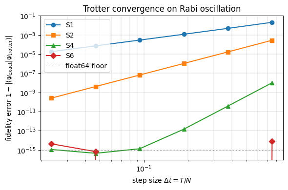

The lines on the plot have slopes $\approx 2, 4, 8$ , matching the fidelity-error orders in the table above. $S_4$ hits the float64 floor already at $N = 16$ ; $S_6$ is at the floor across the entire sweep, so its line appears flat (the expected $\Delta t^{12}$ slope is not resolvable on this 1-qubit problem in double precision).

Summary¶

Model: a single-qubit Rabi Hamiltonian $H = H_z + H_x$ whose non-zero commutator makes Trotter error measurable.
Vector[Observable] + pauli_evolve: the natural primitive for time-stepping; binding the Hamiltonian list at transpile time expands any iteration over Hs.shape[0] into per-term evolutions.
Suzuki–Trotter fractal: $S_{2k}$ is built by nesting five rescaled copies of $S_{2k-2}$ using the level-specific coefficient $p_k = 1/(4 - 4^{1/(2k-1)})$ . Reusing one constant across levels is a common trap and does not produce the fractal.
Recursion: write the math directly as a self-recursive @qkernel with order: UInt. The transpiler iterates inline + partial-eval under a concrete order binding and emits a flat circuit. Without a binding the self-call survives in the IR; non-terminating recursion raises FrontendTransformError.
Convergence: fidelity-error slopes of $2, 4, 8$ on log-log match textbook Trotter orders, and the symbolic dt / n_steps parameters let you sweep step sizes without rebuilding the circuit structure.

Hamiltonian Simulation with Suzuki–Trotter (Rabi oscillation)

The Rabi Hamiltonian¶

Exact reference state¶

S1S_1S1​: First-order Suzuki–Trotter decomposition (Lie–Trotter)¶

S2S_2S2​: Second-order Suzuki–Trotter decomposition (Strang splitting)¶