Möttönen Amplitude Encoding

Tags: algorithm encoding primitive

Amplitude encoding is the operation that, given a unit-norm complex vector $a \in \mathbb{C}^{2^n}$ , prepares the $n$ -qubit state

|\psi\rangle \;=\; \sum_{i=0}^{2^n - 1} a_i \, |i\rangle

(1)

starting from $|0\rangle^{\otimes n}$ . It is the entry door for any algorithm that consumes classical data as a quantum state — including HHL-style linear-system solvers, kernel methods, and many quantum simulation protocols. Qamomile ships a backend-portable implementation under qamomile.circuit.algorithm.state_preparation, based on the uniformly controlled rotation construction of Möttönen, Vartiainen, Bergholm and Salomaa Mottonen et al., 2004 (the paper covers the more general arbitrary-state $|a\rangle \to |b\rangle$ transformation; the implementation only emits the state-preparation half with the input fixed to $|0\rangle^{\otimes n}$ — see §3 on resource estimation for the cost-side consequences).

The construction has two stages:

A cascade of $n$ uniformly controlled $R_y$ gates that distributes the magnitude $|a_i|$ across the basis states. This stage alone is sufficient for real (signed) amplitude vectors.
A second cascade of uniformly controlled $R_z$ gates that restores the relative phases. Only emitted when the input has a non-zero imaginary part.

Each uniformly controlled rotation is decomposed into elementary RY / RZ and CNOT gates using the Gray-code recipe of Möttönen-Vartiainen. The total cost is

Stage	Real input	Complex input
$R_y$ rotations	$2^n - 1$	$2^n - 1$
$R_z$ rotations	0	$2^n - 1$
`CNOT`	$2^n - 2$	$2 (2^n - 2)$

This tutorial walks through the simplest call (§1, §2), then IR visualisation and resource estimation (§3), the runtime-rebindable angles API (§4), and finally embedding into a larger kernel (§5).

⚠️ Pre-condition: the input qubits must be in the all-zero state $|0\rangle^{\otimes n}$ . Qamomile’s amplitude_encoding(...) / amplitude_encoding_from_angles(...) only emits the unitary that maps $|0\rangle^{\otimes n}$ to the target $|\psi\rangle$ (the general Möttönen construction extends to arbitrary inputs, but the implementation specialises to the state-preparation half). Applied to any other input it produces a different output, not the target amplitude vector. Qamomile does not track qubit states at runtime, so it is the caller’s responsibility to invoke these functions immediately after qmc.qubit_array(n, ...), before any other gates touch the register.

import numpy as np
from qiskit.quantum_info import Statevector

import qamomile.circuit as qmc
import qamomile.observable as qm_o
from qamomile.circuit.algorithm import (
    amplitude_encoding,
    amplitude_encoding_from_angles,
)
from qamomile.linalg import (
    compute_mottonen_amplitude_encoding_ry_angles,
    compute_mottonen_amplitude_encoding_rz_angles,
)
from qamomile.qiskit import QiskitTranspiler

transpiler = QiskitTranspiler()
executor = transpiler.executor()

ATOL_STATEVECTOR = 1e-8
ATOL_SHOT = 0.05  # for 8192 shots, ~5σ on p(1-p)/N for any single bin


def fidelity(prepared: np.ndarray, target: np.ndarray) -> float:
    """Phase-invariant fidelity ``|<prepared|target>|^2``."""
    return float(np.abs(np.vdot(prepared, target)) ** 2)


def normalize(amps: list[float] | list[complex]) -> np.ndarray:
    """Unit-norm copy of *amps* (complex dtype if any element is complex)."""
    if any(isinstance(x, complex) for x in amps):
        arr = np.asarray(amps, dtype=complex)
    else:
        arr = np.asarray(amps, dtype=float)
    return arr / np.linalg.norm(arr)


def statevector_of(kernel: qmc.QKernel, **bindings) -> np.ndarray:
    """Run *kernel* through Qiskit's statevector simulator and return the data."""
    qc = transpiler.to_circuit(kernel, bindings=bindings or None)
    return Statevector.from_instruction(
        qc.remove_final_measurements(inplace=False)
    ).data

1. The simplest call — concrete real amplitudes¶

amplitude_encoding(qubits, amplitudes) is the everyday entry point. It accepts a Python sequence or NumPy array, normalises it automatically, and prepares the corresponding state.

As a first sanity check we encode the (un-normalised) vector $a = (1, 2, 3, 4)$ on a 2-qubit register, read back the simulator’s statevector, and assert it matches the normalised target up to phase.

amps_real = [1.0, 2.0, 3.0, 4.0]


@qmc.qkernel
def prepare_real() -> qmc.Vector[qmc.Bit]:
    q = qmc.qubit_array(2, "q")
    q = amplitude_encoding(q, amps_real)
    return qmc.measure(q)


sv = statevector_of(prepare_real)
expected = normalize(amps_real)
print(f"prepared      = {np.round(sv, 4)}")
print(f"target (norm) = {np.round(expected, 4)}")
print(f"fidelity      = {fidelity(sv, expected):.6f}")
assert fidelity(sv, expected) == np.float64(1.0) or np.isclose(
    fidelity(sv, expected), 1.0, atol=ATOL_STATEVECTOR
), "real amplitude encoding lost fidelity"

prepared      = [0.1826+0.j 0.3651+0.j 0.5477+0.j 0.7303+0.j]
target (norm) = [0.1826 0.3651 0.5477 0.7303]
fidelity      = 1.000000

Negative real amplitudes flow through the magnitude stage naturally — the leaf-level $R_y$ angle is taken as a signed arctan2, so the sign is captured without an extra phase stage. The state $a = (1, -1, 1, -1)$ is therefore prepared with RY and CNOT only.

amps_signed = [1.0, -1.0, 1.0, -1.0]


@qmc.qkernel
def prepare_signed() -> qmc.Vector[qmc.Bit]:
    q = qmc.qubit_array(2, "q")
    q = amplitude_encoding(q, amps_signed)
    return qmc.measure(q)


sv = statevector_of(prepare_signed)
expected = normalize(amps_signed)
print(f"fidelity (signed) = {fidelity(sv, expected):.6f}")
assert np.isclose(fidelity(sv, expected), 1.0, atol=ATOL_STATEVECTOR), (
    "signed real encoding lost fidelity"
)

fidelity (signed) = 1.000000

2. Complex amplitudes¶

The same API accepts complex inputs. When at least one entry has a non-zero imaginary part, the implementation switches to the two-stage (Ry + Rz) construction automatically. A complex vector with identically zero imaginary part is silently coerced to the cheaper real path.

We encode $a = (1, 1+i, 1-i, 2i)$ — a generic complex 2-qubit state — and assert the resulting statevector matches (up to global phase).

amps_complex = [1 + 0j, 1 + 1j, 1 - 1j, 0 + 2j]


@qmc.qkernel
def prepare_complex() -> qmc.Vector[qmc.Bit]:
    q = qmc.qubit_array(2, "q")
    q = amplitude_encoding(q, amps_complex)
    return qmc.measure(q)


sv = statevector_of(prepare_complex)
expected = normalize(amps_complex)
print(f"fidelity (complex) = {fidelity(sv, expected):.6f}")
assert np.isclose(fidelity(sv, expected), 1.0, atol=ATOL_STATEVECTOR), (
    "complex encoding lost fidelity"
)

fidelity (complex) = 1.000000

3. Visualisation and resource estimation¶

Drawing the circuit — `kernel.draw()`¶

kernel.draw(fold_loops=False) renders the kernel’s IR. For kernels that use amplitude_encoding, the entire encoding stays as a single MottonenAmplitudeEncoding composite gate in the IR, so by default it shows up as one large opaque box.

prepare_real.draw(fold_loops=False)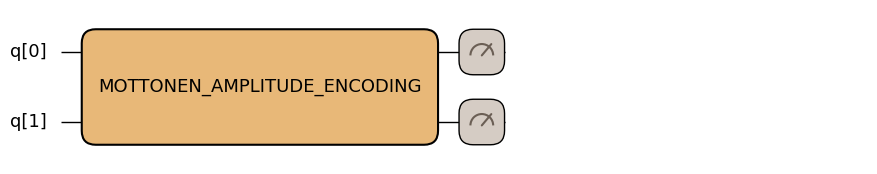

To peek inside, pass expand_composite=True. The composite gate is expanded and the underlying elementary RY / RZ / CNOT gates become visible.

The real path uses only RY and CNOT:

prepare_real.draw(fold_loops=False, expand_composite=True)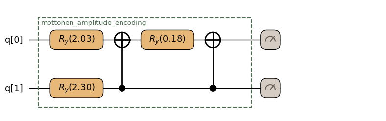

The complex path adds RZ gates at the same positions — you can see them appear in the diagram below:

prepare_complex.draw(fold_loops=False, expand_composite=True)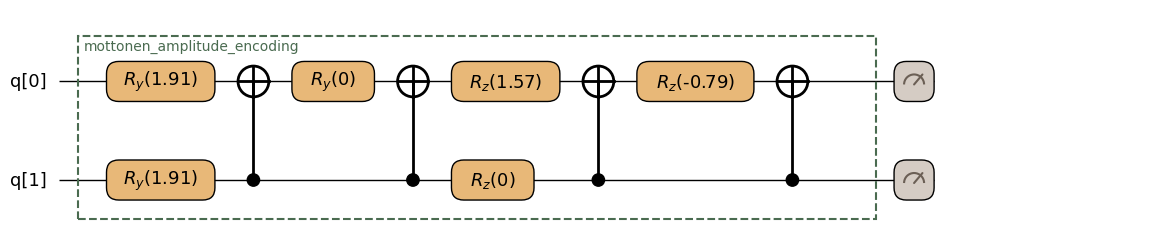

Resource estimation — verifying against the published formula¶

Möttönen, Vartiainen, Bergholm and Salomaa Mottonen et al., 2004 give an explicit closed form for the Gray-code decomposition (Section II, Fig. 2 + paragraph after Eq. (2) — the paper does not number this as a Lemma / Theorem): a $k$ -controlled uniformly controlled rotation costs $2^k$ elementary rotations and $2^k$ CNOTs. Summing over the $n$ stages of the amplitude-encoding cascade — stage $k$ for $k = 0, 1, \ldots, n-1$ , with stage 0 uncontrolled (and therefore CNOT-free) — yields per cascade:

input	rotations	CNOTs
real	$2^n - 1$	$2^n - 2$
complex	$2 \cdot (2^n - 1)$	$2 \cdot (2^n - 2)$

About the discrepancy with the paper’s abstract. The abstract advertises $2^{n+2} - 5$ rotations + $2^{n+2} - 4n - 4$ CNOTs, but that is the cost of the full arbitrary-input → arbitrary-output state transformation $|a\rangle \to |b\rangle$ (decomposed as $|a\rangle \to |e_1\rangle \to |b\rangle$ ). Qamomile’s amplitude_encoding only emits the $|0\rangle^{\otimes n} \to |\psi\rangle$ half, so the table above is roughly half that cost. Note that the implementation also does not apply inter-cascade CNOT cancellation — it sticks with the plain per-stage decomposition.

We verify that kernel.estimate_resources() reports exactly these numbers across a range of register sizes. This walks the full composite-gate-aware estimator path (not just the MottonenAmplitudeEncoding._resources() metadata directly) so the check also exercises the IR resolution.

def make_real_kernel(n: int) -> qmc.QKernel:
    """Build a kernel that runs the real-input Möttönen path on ``n`` qubits."""
    real_amps = np.ones(2**n).tolist()

    @qmc.qkernel
    def kernel() -> qmc.Vector[qmc.Bit]:
        q = qmc.qubit_array(n, "q")
        q = amplitude_encoding(q, real_amps)
        return qmc.measure(q)

    return kernel


def make_complex_kernel(n: int) -> qmc.QKernel:
    """Build a kernel that runs the complex (Ry+Rz) Möttönen path."""
    cplx_amps = (np.ones(2**n) + 1j * np.arange(2**n)).tolist()

    @qmc.qkernel
    def kernel() -> qmc.Vector[qmc.Bit]:
        q = qmc.qubit_array(n, "q")
        q = amplitude_encoding(q, cplx_amps)
        return qmc.measure(q)

    return kernel


print(f"{'n':>3s} | {'real(rot/CNOT)':>16s} | {'complex(rot/CNOT)':>20s}")
print(f"{'---':>3s} | {'---':>16s} | {'---':>20s}")
for n in (2, 3, 4, 5):
    er = make_real_kernel(n).estimate_resources()
    ec = make_complex_kernel(n).estimate_resources()
    rot_real, cnot_real = int(er.gates.rotation_gates), int(er.gates.two_qubit)
    rot_cplx, cnot_cplx = int(ec.gates.rotation_gates), int(ec.gates.two_qubit)
    print(
        f"{n:>3d} | {f'{rot_real} / {cnot_real}':>16s} | {f'{rot_cplx} / {cnot_cplx}':>20s}"
    )

    # Möttönen-Vartiainen closed form, asserted directly:
    assert rot_real == 2**n - 1, f"real rotations off at n={n}"
    assert cnot_real == 2**n - 2, f"real CNOTs off at n={n}"
    assert rot_cplx == 2 * (2**n - 1), f"complex rotations off at n={n}"
    assert cnot_cplx == 2 * (2**n - 2), f"complex CNOTs off at n={n}"

  n |   real(rot/CNOT) |    complex(rot/CNOT)
--- |              --- |                  ---
  2 |            3 / 2 |                6 / 4
  3 |            7 / 6 |              14 / 12
  4 |          15 / 14 |              30 / 28
  5 |          31 / 30 |              62 / 60

Both rotation and CNOT counts grow as $O(2^n)$ in $n$ — amplitude encoding is intrinsically expensive for many qubits.

4. Runtime-rebindable angles API¶

The state-preparation package exposes two main user-facing entry points:

amplitude_encoding(q, amplitudes) — the amplitude-based entry used in §1–§3. Computes Möttönen angles from the amplitudes at compile time and leaves a single MottonenAmplitudeEncoding composite gate in the IR.
amplitude_encoding_from_angles(q, ry_angles, rz_angles=None) — the angle-based entry, which takes Möttönen angles pre-computed by the caller. This is the only path that lets a single compiled circuit be re-bound at run time to many different amplitude vectors (hybrid optimisation loops, parameter sweeps).

amplitude_encoding further supports passing the amplitudes either as (a) a concrete sequence directly, or (b) a Vector[Float] kernel parameter resolved at compile time via bindings={...}. The next two subsections exercise (b) and amplitude_encoding_from_angles — everything that was not already shown in §1–§3.

4.1 `amplitude_encoding` with a bound `Vector[Float]` parameter¶

When you’d rather not bake the amplitudes in as a magic number (sweeping, exposing them as documentation, ...), declare amps: Vector[Float] as a kernel parameter and pass values via bindings={"amps": [...]}. The bound concrete data is read at trace time, so the IR shape is identical to the concrete-sequence form from §1. Real-only (a Vector[Float] cannot carry complex values).

@qmc.qkernel
def prepare_via_binding(amps: qmc.Vector[qmc.Float]) -> qmc.Vector[qmc.Bit]:
    q = qmc.qubit_array(2, "q")
    q = amplitude_encoding(q, amps)
    return qmc.measure(q)


prepare_via_binding.draw(fold_loops=False, amps=[1.0, 2.0, 3.0, 4.0])

sv = statevector_of(prepare_via_binding, amps=[1.0, 2.0, 3.0, 4.0])
print(
    f"fidelity (bound Vector[Float]) = {fidelity(sv, normalize([1.0, 2.0, 3.0, 4.0])):.6f}"
)
assert np.isclose(
    fidelity(sv, normalize([1.0, 2.0, 3.0, 4.0])), 1.0, atol=ATOL_STATEVECTOR
)

fidelity (bound Vector[Float]) = 1.000000

Trying to leave that parameter symbolic with parameters=["amps"] is rejected with a directing error — the angle computation (atan2(|a_1|, |a_0|) and friends) needs concrete numbers and therefore fundamentally cannot be deferred to runtime. The error points at amplitude_encoding_from_angles for the runtime case.

try:
    transpiler.transpile(prepare_via_binding, parameters=["amps"])
except ValueError as exc:
    print(f"ValueError: {exc}")
    raised = True
else:
    raised = False
assert raised, "expected ValueError when amps is a runtime parameter"

ValueError: amplitude_encoding received a Vector[Float] handle without concrete values at trace time. Bind it via transpiler.transpile(kernel, bindings={...}) for compile-time amplitudes, or use amplitude_encoding_from_angles with parameters=[...] for runtime-parametric angles.

4.2 `amplitude_encoding_from_angles` — compile once, re-bind many times¶

amplitude_encoding_from_angles is the only path that lets us reuse a single compiled circuit across different amplitude vectors at run time. Pre-compute the angles classically with the compute_mottonen_amplitude_encoding_*_angles helpers, transpile once with parameters=[...], then sample with new bindings each iteration. Complex inputs are supported (just pass rz_angles).

Note: this path skips the MottonenAmplitudeEncoding composite-gate wrapping and emits the elementary RY / RZ / CNOT gates directly into the IR — resource estimation sees the elementary gates rather than the high-level op.

@qmc.qkernel
def prepare_from_angles(
    ry_a: qmc.Vector[qmc.Float], rz_a: qmc.Vector[qmc.Float]
) -> qmc.Vector[qmc.Bit]:
    q = qmc.qubit_array(2, "q")
    q = amplitude_encoding_from_angles(q, ry_a, rz_a)
    return qmc.measure(q)


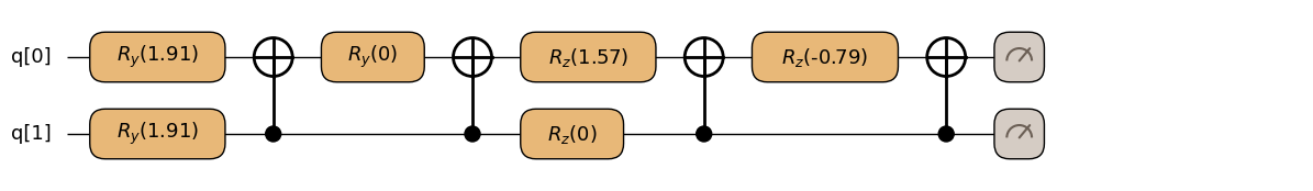
prepare_from_angles.draw(
    fold_loops=False,
    ry_a=compute_mottonen_amplitude_encoding_ry_angles(amps_complex).tolist(),
    rz_a=compute_mottonen_amplitude_encoding_rz_angles(amps_complex).tolist(),
)

exe = transpiler.transpile(prepare_from_angles, parameters=["ry_a", "rz_a"])
n_runtime_params = len(exe.compiled_quantum[0].circuit.parameters)
print(f"runtime parameters in compiled circuit: {n_runtime_params}")
assert n_runtime_params == 2 * (2**2 - 1), (
    "expected 2 * (2^n - 1) parametric rotations for n=2 complex"
)

shots = 8192
for trial_amps in (
    [1.0, 0.0, 0.0, 1.0],
    [3.0, 4.0, 0.0, 0.0],
    [1 + 0j, 1j, -1 + 0j, -1j],
):
    ry = compute_mottonen_amplitude_encoding_ry_angles(trial_amps).tolist()
    rz = compute_mottonen_amplitude_encoding_rz_angles(trial_amps).tolist()
    counts = (
        exe.sample(executor, shots=shots, bindings={"ry_a": ry, "rz_a": rz})
        .result()
        .results
    )
    observed = np.zeros(4)
    for bits, c in counts:
        idx = sum(int(b) << i for i, b in enumerate(bits))
        observed[idx] = c / shots
    expected_probs = np.abs(normalize(trial_amps)) ** 2
    max_dev = float(np.max(np.abs(observed - expected_probs)))
    print(f"amps={str(trial_amps):<48s}  max|p_obs - p_exp| = {max_dev:.4f}")
    assert max_dev < ATOL_SHOT, (
        f"runtime-parametric sampling diverged for amps={trial_amps}"
    )

runtime parameters in compiled circuit: 6
amps=[1.0, 0.0, 0.0, 1.0]                              max|p_obs - p_exp| = 0.0024
amps=[3.0, 4.0, 0.0, 0.0]                              max|p_obs - p_exp| = 0.0021
amps=[(1+0j), 1j, (-1+0j), (-0-1j)]                    max|p_obs - p_exp| = 0.0040

All three iterations sample from the same compiled circuit; only the runtime bindings change. The maximum per-bin deviation stays within shot-noise tolerance.

5. Plugging into a larger kernel — observable estimation¶

amplitude_encoding is a building block — most users plug it into a larger kernel. The simplest such use case is computing $\langle \psi | H | \psi \rangle$ for some Hamiltonian $H$ on the prepared state. The kernel becomes a single expval, and the observable can be passed in as a runtime binding.

As a small analytic check, the encoded state for $a = (1, 2, 3, 4)$ (little-endian, qubit 0 = LSB) gives

\langle Z_0 \rangle = (p_{00} + p_{10}) - (p_{01} + p_{11}) = \frac{1 + 9 - 4 - 16}{30} = -\tfrac{1}{3},

(2)

which we now reproduce with the estimator path.

@qmc.qkernel
def expval_kernel(H: qmc.Observable) -> qmc.Float:
    q = qmc.qubit_array(2, "q")
    q = amplitude_encoding(q, [1.0, 2.0, 3.0, 4.0])
    return qmc.expval(q, H)


H = qm_o.Z(0) + 0.0 * qm_o.Z(1)  # pad to 2-qubit width
exe_expval = transpiler.transpile(expval_kernel, bindings={"H": H})
result = exe_expval.run(executor).result()
print(f"<Z_0> = {float(result):+.6f}   (analytic: {-1 / 3:+.6f})")
assert np.isclose(float(result), -1.0 / 3.0, atol=1e-8), (
    "<Z_0> estimator deviated from analytic value"
)

<Z_0> = -0.333333   (analytic: -0.333333)

Summary — which API for which use case¶

Goal	Use
You have the amplitudes as a Python list / NumPy array (most common)	`amplitude_encoding(q, [...])` (§1, §2)
Expose the amplitudes as a kernel parameter, bind at compile time (real only)	`amplitude_encoding(q, amps)` + `bindings={"amps": [...]}` (§4.1)
Reuse one compiled circuit across many amplitude vectors at run time (sweeps, hybrid optimisation)	`amplitude_encoding_from_angles(q, ry, rz)` + `parameters=[...]` (§4.2)
Pre-compute the angles classically (caching, sharing across kernels, inspection)	`compute_mottonen_amplitude_encoding_{ry,rz}_angles(amps)` (`qamomile.linalg`)

When in doubt, start with amplitude_encoding(q, [...]) and switch to amplitude_encoding_from_angles only when you actually need run-time rebinding — that is the typical evolution path.

References¶

Mottonen, M., Vartiainen, J. J., Bergholm, V., & Salomaa, M. M. (2004). Transformation of quantum states using uniformly controlled rotations. 10.48550/ARXIV.QUANT-PH/0407010