QAOA for Graph Partitioning - Qamomile Documentation

Tags: algorithm optimization variational

This tutorial demonstrates how to solve the graph partitioning problem using the Quantum Approximate Optimization Algorithm (QAOA) with Qamomile.

The workflow is:

JijModeling problem → problem.eval() → QAOAConverter → transpile → sample → decode

Formulate the problem with JijModeling.
Create an instance with concrete data.
Use QAOAConverter to build the QAOA circuit and Hamiltonian.
Optimize the variational parameters with a classical optimizer.
Sample the optimized circuit and decode the results.

# Install the latest Qamomile through pip!
# !pip install qamomile

Problem Formulation¶

Given an undirected graph $G = (V, E)$ , the goal is to partition the vertices into two groups of equal size while minimizing the number of edges between the two groups.

Objective:

\min \sum_{(u,v) \in E} \bigl[x_u(1 - x_v) + x_v(1 - x_u)\bigr]

(1)

Constraint:

\sum_{u \in V} x_u = \frac{|V|}{2}

(2)

where $x_u \in \{0, 1\}$ indicates which partition vertex $u$ belongs to.

Define the Problem with JijModeling¶

import jijmodeling as jm

problem = jm.Problem("Graph Partitioning")


@problem.update
def _(problem: jm.DecoratedProblem):
    V = problem.Dim()
    E = problem.Natural(ndim=2)  # edge list: [[u1,v1], [u2,v2], ...]
    x = problem.BinaryVar(shape=(V,))

    # Objective: minimize edges cut between partitions
    problem += (
        E.rows().map(lambda e: x[e[0]] * (1 - x[e[1]]) + x[e[1]] * (1 - x[e[0]])).sum()
    )

    # Constraint: equal partition sizes
    problem += problem.Constraint("Equal Partition", x.sum() == V / 2)


problem

Graph Instance¶

We use a fixed 8-node graph with 16 edges for reproducibility.

import matplotlib.pyplot as plt
import networkx as nx

num_nodes = 8
edge_list = [
    [0, 2],
    [0, 3],
    [0, 4],
    [1, 2],
    [1, 3],
    [1, 4],
    [1, 5],
    [1, 7],
    [2, 3],
    [2, 6],
    [3, 5],
    [4, 5],
    [4, 6],
    [5, 6],
    [5, 7],
    [6, 7],
]

G = nx.Graph()
G.add_nodes_from(range(num_nodes))
G.add_edges_from(edge_list)

pos = nx.spring_layout(G, seed=1)
plt.figure(figsize=(5, 5))
nx.draw(
    G,
    pos,
    with_labels=True,
    node_color="white",
    node_size=700,
    edgecolors="black",
)
plt.title(f"Graph: {G.number_of_nodes()} nodes, {G.number_of_edges()} edges")
plt.show()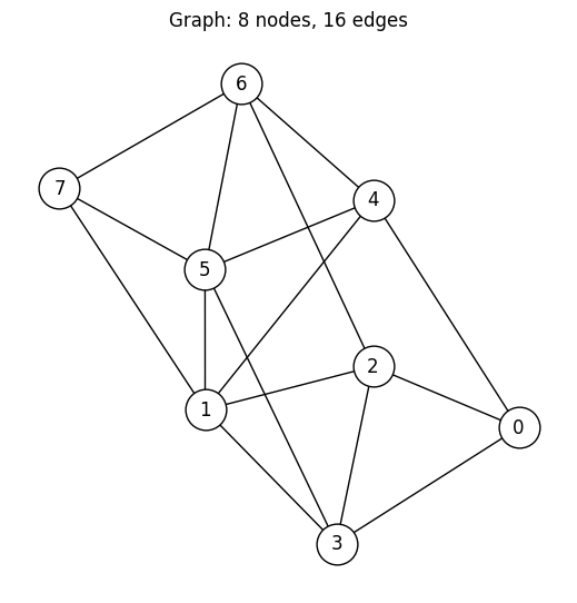

Create the Instance¶

We extract the edge list from the graph and evaluate the JijModeling problem with the concrete data.

instance_data = {"V": num_nodes, "E": edge_list}
instance = problem.eval(instance_data)

Set Up the QAOAConverter¶

QAOAConverter takes an OMMX instance and internally:

Converts the problem to a QUBO (Quadratic Unconstrained Binary Optimization) form.
Transforms from BINARY variables to SPIN variables.
Builds the cost Hamiltonian as a sum of Pauli-Z operators.

Because the original problem has a constraint, the QUBO formulation folds it into the objective as a penalty term. This means the energy values from the decoded samples are not the original objective (number of cut edges) — they include the penalty. We will need to check feasibility and compute the true objective separately.

from qamomile.optimization.qaoa import QAOAConverter

converter = QAOAConverter(instance)
converter.spin_model = converter.spin_model.normalize_by_abs_max()
hamiltonian = converter.get_cost_hamiltonian()
print(hamiltonian)

Hamiltonian((Z0, Z1): 1.0, (Z0, Z5): 1.0, (Z0, Z6): 1.0, (Z0, Z7): 1.0, (Z1, Z6): 1.0, (Z2, Z4): 1.0, (Z2, Z5): 1.0, (Z2, Z7): 1.0, (Z3, Z4): 1.0, (Z3, Z6): 1.0, (Z3, Z7): 1.0, (Z4, Z7): 1.0)

Transpile to an Executable Circuit¶

converter.transpile() builds a QAOA ansatz circuit with p layers and compiles it into an ExecutableProgram. The variational parameters gammas (cost layer) and betas (mixer layer) remain as runtime parameters.

from qamomile.qiskit import QiskitTranspiler

transpiler = QiskitTranspiler()
p = 5  # number of QAOA layers
executable = converter.transpile(transpiler, p=p)

Visualize the QAOA Circuit¶

QAOAConverter._transpile_quadratic() internally builds the sampling qkernel below and feeds it to the transpiler. For visualization we restate that qkernel verbatim, then trace it through the early pipeline (Transpiler.to_block to lower it into an IR Block, Transpiler.inline to expand the sub-qkernel calls) before handing the resulting Block to MatplotlibDrawer.draw. This renders exactly the Block structure the converter works with internally, with p=2 for readability.

import qamomile.circuit as qmc
from qamomile.circuit.algorithm.qaoa import qaoa_state
from qamomile.circuit.visualization import MatplotlibDrawer


@qmc.qkernel
def qaoa_sampling(
    p: qmc.UInt,
    quad: qmc.Dict[qmc.Tuple[qmc.UInt, qmc.UInt], qmc.Float],
    linear: qmc.Dict[qmc.UInt, qmc.Float],
    gammas: qmc.Vector[qmc.Float],
    betas: qmc.Vector[qmc.Float],
    n: qmc.UInt,
) -> qmc.Vector[qmc.Bit]:
    q = qaoa_state(p=p, quad=quad, linear=linear, n=n, gammas=gammas, betas=betas)
    return qmc.measure(q)


block = transpiler.to_block(
    qaoa_sampling,
    bindings={
        "linear": converter.spin_model.linear,
        "quad": converter.spin_model.quad,
        "n": converter.spin_model.num_bits,
        "p": 2,
    },
    parameters=["gammas", "betas"],
)
block = transpiler.inline(block)
# `fold_loops=False` unrolls every loop (`for layer`,
# `for (i,j),Jij in quad`, and the per-qubit range loops) so each gate
# is rendered explicitly. `linear` is the empty dict `{}` for graph
# partition (no linear Ising terms), so its ForItems loop has zero
# iterations and is rendered as nothing rather than as a folded box.
# The result is wide; the docs build injects a lightbox script that
# turns each cell-output image into a click-to-zoom modal so the wide
# rendering stays inspectable on ReadTheDocs.
MatplotlibDrawer(block).draw(fold_loops=False)

Inspecting the Building Blocks¶

Inside qaoa_sampling we call qaoa_state, and qaoa_state itself is the composition of three smaller qkernels:

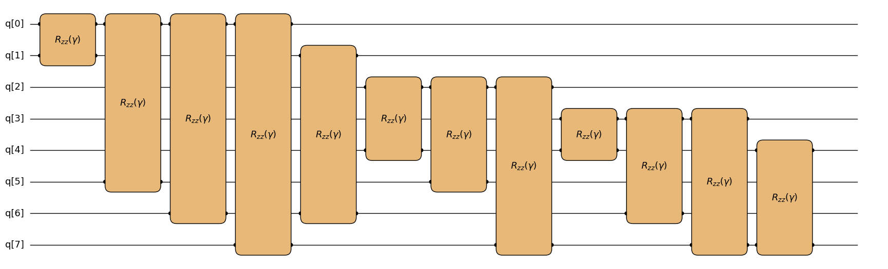
superposition_vector(n) — applies H to every qubit, preparing the initial state $|+\rangle^{\otimes n}$ .
ising_cost(quad, linear, q, gamma) — the cost layer: one RZZ per quadratic entry in quad and one RZ per linear entry in linear. The graph-partition spin model has no linear terms (linear={}), so only RZZ gates appear.
x_mixer(q, beta) — the mixer layer: applies RX(2\beta) to every qubit.

qaoa_layers(p, ...) is just the alternation of ising_cost and x_mixer, repeated p times. Below we render each piece on its own.

from qamomile.circuit.algorithm.basic import superposition_vector
from qamomile.circuit.algorithm.qaoa import ising_cost, x_mixer

superposition_vector.draw(n=converter.spin_model.num_bits, fold_loops=False)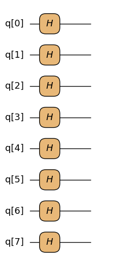

ising_cost.draw(
    q=converter.spin_model.num_bits,
    quad=converter.spin_model.quad,
    linear=converter.spin_model.linear,
    fold_loops=False,
)

x_mixer.draw(q=converter.spin_model.num_bits, fold_loops=False)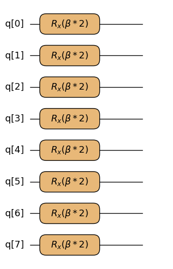

Optimize the QAOA Parameters¶

We use executable.sample() to evaluate the cost at each iteration of the classical optimizer. The optimizer explores different gammas and betas to minimize the mean energy of the sampled bitstrings.

import os

import numpy as np
from qiskit_aer import AerSimulator
from scipy.optimize import minimize

# Seed the simulator so re-executing the notebook reproduces the same
# COBYLA trajectory and final sampling distribution. Without a seed,
# every shot draws fresh randomness, COBYLA sees a noisy cost surface,
# and each notebook run converges to a different (but equivalent) local
# optimum.
executor = transpiler.executor(
    backend=AerSimulator(seed_simulator=901, max_parallel_threads=1)
)
docs_test_mode = os.environ.get("QAMOMILE_DOCS_TEST") == "1"
sample_shots = 256 if docs_test_mode else 2048
maxiter = 25 if docs_test_mode else 1000

rng = np.random.default_rng(900)
initial_params = rng.uniform(0, np.pi, 2 * p)

cost_history = []


def cost_fn(params):
    gammas = list(params[:p])
    betas = list(params[p:])
    job = executable.sample(
        executor,
        shots=sample_shots,
        bindings={"gammas": gammas, "betas": betas},
    )
    result = job.result()
    # decode_to_binary_sampleset returns the QUBO-domain BinarySampleSet
    # whose `energy` is the penalized objective — what COBYLA needs to
    # see infeasibility costs. The polymorphic decode() returns an
    # ommx.v1.SampleSet whose `objective` is the un-penalized true
    # objective; using it here would let the optimizer settle on
    # infeasible all-zero / all-one bitstrings.
    decoded = converter.decode_to_binary_sampleset(result)
    energy = decoded.energy_mean()
    cost_history.append(energy)
    return energy


res = minimize(
    cost_fn,
    initial_params,
    method="COBYLA",
    options={"maxiter": maxiter},
)

print(f"Optimized cost: {res.fun:.3f}")
print(f"Optimal params: {[round(v, 4) for v in res.x]}")
print(f"Function evaluations: {res.nfev}")

Optimized cost: 14.235
Optimal params: [np.float64(0.5042), np.float64(0.9744), np.float64(3.1558), np.float64(0.7789), np.float64(2.1748), np.float64(1.1239), np.float64(3.6516), np.float64(1.5606), np.float64(1.5563), np.float64(0.7607)]
Function evaluations: 117

plt.figure(figsize=(8, 4))
plt.plot(cost_history, color="#2696EB")
plt.xlabel("Iteration")
plt.ylabel("Cost (mean energy)")
plt.title("QAOA Optimization Progress")
plt.show()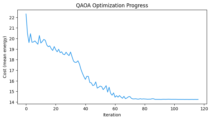

Sample with Optimized Parameters¶

With the optimized parameters, we sample the circuit to collect candidate solutions as bitstrings.

gammas_opt = list(res.x[:p])
betas_opt = list(res.x[p:])

sample_result = executable.sample(
    executor,
    shots=1000,
    bindings={"gammas": gammas_opt, "betas": betas_opt},
).result()

# `decode()` on an OMMX-backed converter returns an `ommx.v1.SampleSet`
# evaluated against the *original* (un-penalized) instance, so
# feasibility, the true objective, and per-constraint diagnostics are
# available through OMMX's own API — no hand-rolled feasibility or
# objective helper is needed.
sample_set = converter.decode(sample_result)

Analyze the Results¶

Feasibility Check¶

QAOA samples are candidate solutions — they are not guaranteed to satisfy the original constraints. The constraint $\sum x_u = |V|/2$ was folded into the QUBO as a penalty, so infeasible bitstrings can still appear in the output.

SampleSet.summary is a DataFrame with one row per shot whose feasible column already encodes feasibility against the original constraints, so we can read the feasible-shot count straight off it.

summary = sample_set.summary
total_feasible = int(summary["feasible"].sum())
total_samples = len(summary)

print(
    f"Feasible samples: {total_feasible} / {total_samples} "
    f"({100 * total_feasible / total_samples:.1f}%)"
)

Feasible samples: 538 / 1000 (53.8%)

Best Feasible Solution¶

SampleSet.best_feasible returns the feasible sample with the best (here: smallest) objective. Because the converter was built from an OMMX Instance, the reported objective is the original un-penalized one — i.e. the number of cut edges itself — and the decision-variable values come back keyed by the original variable IDs in decision_variables_df.

if total_feasible > 0:
    best = sample_set.best_feasible
    best_obj = int(round(best.objective))
    best_sample = {
        i: int(round(best.decision_variables_df.loc[i, "value"]))
        for i in range(num_nodes)
    }
    print(f"Best feasible solution: {best_sample}")
    print(f"Cut edges:             {best_obj}")
else:
    print("No feasible solution found. Try increasing p or maxiter.")
    best_sample = None
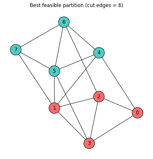
    best_obj = None

Best feasible solution: {0: 1, 1: 1, 2: 1, 3: 1, 4: 0, 5: 0, 6: 0, 7: 0}
Cut edges:             6

Objective Value Distribution¶

We plot the distribution of the true objective value (cut edges) for feasible samples only. summary already has the original objective per shot, so a value_counts() on the feasible slice gives the histogram directly.

if total_feasible > 0:
    feasible_objectives = (
        summary.loc[summary["feasible"], "objective"].round().astype(int)
    )
    obj_counts = feasible_objectives.value_counts().sort_index()

    plt.figure(figsize=(8, 4))
    plt.bar([str(o) for o in obj_counts.index], obj_counts.values, color="#2696EB")
    plt.xlabel("Cut edges (objective value)")
    plt.ylabel("Frequency")
    plt.title("Distribution of Feasible Solutions")
    plt.show()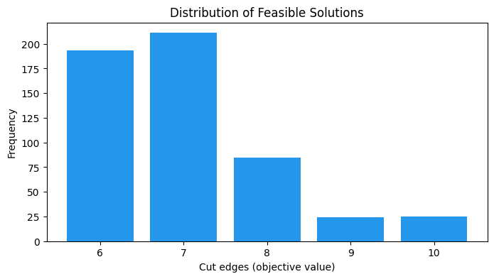

Visualize the Best Partition¶

We color the graph nodes according to the best feasible partition found by QAOA.

if best_sample is not None:
    color_map = [
        "#FF6B6B" if best_sample.get(i, 0) == 1 else "#4ECDC4" for i in range(num_nodes)
    ]

    plt.figure(figsize=(5, 5))
    nx.draw(
        G,
        pos,
        with_labels=True,
        node_color=color_map,
        node_size=700,
        edgecolors="black",
    )
    plt.title(f"Best feasible partition (cut edges = {best_obj})")
    plt.show()