QAOA for MaxCut: Building the Circuit from Scratch

Tags: algorithm optimization variational

This tutorial walks through the Quantum Approximate Optimization Algorithm (QAOA) pipeline step by step, using Qamomile’s low-level circuit primitives. Rather than using the high-level QAOAConverter, we will:

Define a MaxCut problem for a small graph.
Formulate it directly as an Ising model on spin variables.
Write the QAOA circuit step by step using @qkernel.
Optimize variational parameters with a classical optimizer.
Decode and visualize the results.

At the end, we show that qamomile.circuit.algorithm.qaoa_state provides the same circuit in a single function call.

# Install the latest Qamomile through pip!
# !pip install qamomile

What is MaxCut?¶

Given an undirected graph $G = (V, E)$ , the MaxCut problem asks us to partition the vertices into two sets so that the number of edges crossing between the two sets is maximized.

MaxCut is naturally a spin problem. Assign each vertex $i$ a spin $s_i \in \{+1, -1\}$ indicating which side of the cut it belongs to. An edge $(i, j)$ is cut exactly when $s_i \ne s_j$ , so the number of cut edges is

\text{MaxCut}(\boldsymbol{s}) = \sum_{(i,j) \in E} \frac{1 - s_i s_j}{2}.

(1)

Spin-based problems such as MaxCut, spin-glass ground states, and Ising model benchmarks are most cleanly written in the spin domain. We therefore skip the QUBO / binary encoding detour and work directly with spin variables throughout this tutorial.

Create the Graph¶

We use a small 5-node graph with 6 edges. This is large enough to be non-trivial, yet small enough to brute-force for comparison.

import matplotlib.pyplot as plt
import networkx as nx

G = nx.Graph()
G.add_edges_from([(0, 1), (0, 2), (1, 2), (1, 3), (2, 3), (3, 4)])
num_nodes = G.number_of_nodes()

pos = nx.spring_layout(G, seed=42)
plt.figure(figsize=(5, 4))
nx.draw(
    G,
    pos,
    with_labels=True,
    node_color="white",
    node_size=700,
    edgecolors="black",
)
plt.title(f"Graph: {num_nodes} nodes, {G.number_of_edges()} edges")
plt.show()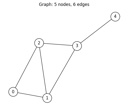

Ising Formulation¶

Maximizing $\sum_{(i,j) \in E} (1 - s_i s_j) / 2$ is equivalent (up to a constant) to minimizing the antiferromagnetic Ising Hamiltonian

H_C(\boldsymbol{s}) = \sum_{(i,j) \in E} s_i s_j.

(2)

Compared to the general Ising form $H = \sum_i h_i s_i + \sum_{i < j} J_{ij} s_i s_j$ , unweighted MaxCut has:

no linear terms: $h_i = 0$ for every vertex, and
uniform couplings: $J_{ij} = 1$ for every edge $(i, j) \in E$ .

BinaryModel.from_ising takes the Ising coefficients directly — there is no need to go through a QUBO and convert variable types.

from qamomile.optimization.binary_model import BinaryModel

ising_quad: dict[tuple[int, int], float] = {
    tuple(sorted((i, j))): 1.0 for i, j in G.edges()
}
ising_linear: dict[int, float] = {}

# For weighted MaxCut or spin-glass instances where the J_{ij} are not all
# of the same magnitude, append `.normalize_by_abs_max()` here to keep the
# cost-landscape scale comparable across runs (helps gradient-free
# optimizers such as COBYLA converge consistently).
spin_model = BinaryModel.from_ising(linear=ising_linear, quad=ising_quad)

print(f"Variable type:          {spin_model.vartype}")
print(f"Linear terms (h_i):     {spin_model.linear}")
print(f"Quadratic terms (J_ij): {spin_model.quad}")
print(f"Constant:               {spin_model.constant}")

Variable type:          SPIN
Linear terms (h_i):     {}
Quadratic terms (J_ij): {(0, 1): 1.0, (0, 2): 1.0, (1, 2): 1.0, (1, 3): 1.0, (2, 3): 1.0, (3, 4): 1.0}
Constant:               0.0

Note: BinaryModel also provides from_qubo() and from_hubo() for problems that are naturally expressed in the binary domain (e.g., assignment problems, constrained problems with penalty terms). See QAOA for Graph Partitioning for a QUBO / JijModeling-based workflow.

Exact Solution (Brute Force)¶

Before running QAOA, let’s find the optimal partition by trying all $2^n = 32$ spin configurations. This gives us a ground truth to compare against.

import itertools

best_cut = 0
optimal_partitions: list[tuple[int, ...]] = []

for spins in itertools.product([+1, -1], repeat=num_nodes):
    cut = sum(1 for i, j in G.edges() if spins[i] != spins[j])
    if cut > best_cut:
        best_cut = cut
        optimal_partitions = [spins]
    elif cut == best_cut:
        optimal_partitions.append(spins)

print(f"Optimal MaxCut value: {best_cut}")
print(f"Number of optimal partitions: {len(optimal_partitions)}")
for part in optimal_partitions:
    print(f"  {part}")

Optimal MaxCut value: 5
Number of optimal partitions: 2
  (1, -1, -1, 1, -1)
  (-1, 1, 1, -1, 1)

QAOA Circuit: The Idea¶

The QAOA ansatz prepares a parameterized quantum state:

|\boldsymbol{\gamma}, \boldsymbol{\beta}\rangle = \prod_{l=1}^{p} e^{-i \beta_l H_M} \, e^{-i \gamma_l H_C} \; |{+}\rangle^{\otimes n}

(3)

where:

$|{+}\rangle^{\otimes n}$ : uniform superposition (Hadamard on every qubit)
$e^{-i \gamma H_C}$ : cost unitary — for the Ising cost $H_C$ , this decomposes into $\text{RZZ}$ gates for quadratic terms and $\text{RZ}$ gates for linear terms (see Steps 2–3 for the gate convention details)
$e^{-i \beta H_M}$ : mixer unitary — with $H_M = \sum_i X_i$ , this becomes $\text{RX}(2\beta)$ on every qubit
$p$ : number of layers (depth of the ansatz)

The spin $\leftrightarrow$ computational-basis correspondence is the standard quantum convention $Z|0\rangle = |0\rangle$ , $Z|1\rangle = -|1\rangle$ , so measurement outcome 0 maps to spin +1 and outcome 1 maps to spin -1.

We will now build each component as a @qkernel.

Step 1: Uniform Superposition¶

Apply a Hadamard gate to every qubit to start from the equal superposition state $|{+}\rangle^{\otimes n}$ .

import qamomile.circuit as qmc


@qmc.qkernel
def superposition(n: qmc.UInt) -> qmc.Vector[qmc.Qubit]:
    q = qmc.qubit_array(n, name="q")
    for i in qmc.range(n):
        q[i] = qmc.h(q[i])
    return q

Step 2: Cost Layer¶

Apply the cost unitary $e^{-i \gamma H_C}$ .

Qamomile’s rotation gates include a $1/2$ factor: $\text{RZ}(\theta) = e^{-i \theta Z / 2}$ and $\text{RZZ}(\theta) = e^{-i \theta Z \otimes Z / 2}$ . To match $e^{-i \gamma H_C}$ exactly one would pass $2 J_{ij} \gamma$ as the angle. However, since $\gamma$ is a variational parameter that the classical optimizer tunes freely, this constant factor is simply absorbed into the optimal $\gamma$ values. We therefore pass $J_{ij} \cdot \gamma$ (and $h_i \cdot \gamma$ ) directly.

We keep the linear argument even though it is empty for unweighted MaxCut — this makes the kernel immediately reusable for weighted MaxCut and generic spin-glass Hamiltonians, which do include linear $h_i$ terms.

@qmc.qkernel
def cost_layer(
    quad: qmc.Dict[qmc.Tuple[qmc.UInt, qmc.UInt], qmc.Float],
    linear: qmc.Dict[qmc.UInt, qmc.Float],
    q: qmc.Vector[qmc.Qubit],
    gamma: qmc.Float,
) -> qmc.Vector[qmc.Qubit]:
    for (i, j), Jij in quad.items():
        q[i], q[j] = qmc.rzz(q[i], q[j], angle=Jij * gamma)
    for i, hi in linear.items():
        q[i] = qmc.rz(q[i], angle=hi * gamma)
    return q

Step 3: Mixer Layer¶

Apply the mixer unitary $e^{-i \beta H_M}$ where $H_M = \sum_i X_i$ . Since $\text{RX}(\theta) = e^{-i \theta X / 2}$ , we need $\theta = 2\beta$ to implement $e^{-i \beta X_i}$ on each qubit.

@qmc.qkernel
def mixer_layer(
    q: qmc.Vector[qmc.Qubit],
    beta: qmc.Float,
) -> qmc.Vector[qmc.Qubit]:
    n = q.shape[0]
    for i in qmc.range(n):
        q[i] = qmc.rx(q[i], angle=2.0 * beta)
    return q

Step 4: Full QAOA Ansatz¶

Compose the three pieces: superposition, then $p$ rounds of cost + mixer, and finally measurement.

@qmc.qkernel
def qaoa_ansatz(
    p: qmc.UInt,
    quad: qmc.Dict[qmc.Tuple[qmc.UInt, qmc.UInt], qmc.Float],
    linear: qmc.Dict[qmc.UInt, qmc.Float],
    n: qmc.UInt,
    gammas: qmc.Vector[qmc.Float],
    betas: qmc.Vector[qmc.Float],
) -> qmc.Vector[qmc.Bit]:
    q = superposition(n)
    for layer in qmc.range(p):
        q = cost_layer(quad, linear, q, gammas[layer])
        q = mixer_layer(q, betas[layer])
    return qmc.measure(q)

Transpile and Optimize¶

We transpile the kernel, binding the problem structure (Ising coefficients, number of qubits, number of layers) while keeping gammas and betas as runtime parameters that the optimizer will tune.

from qamomile.qiskit import QiskitTranspiler

transpiler = QiskitTranspiler()
p = 3  # number of QAOA layers

executable = transpiler.transpile(
    qaoa_ansatz,
    bindings={
        "p": p,
        "quad": spin_model.quad,
        "linear": spin_model.linear,
        "n": num_nodes,
    },
    parameters=["gammas", "betas"],
)

We use scipy.optimize.minimize with the COBYLA method. At each iteration, the optimizer samples the circuit and evaluates the mean energy.

To make the tutorial reproducible we (i) pass seed_simulator=SEED to AerSimulator so the per-shot pseudo-random sampling is deterministic, (ii) seed the NumPy generator with the same value so initial variational parameters are stable, and (iii) set max_parallel_threads=1 so the simulator does not interleave random draws across threads. The single-thread setting trades a little performance for fully reproducible runs; in production code you can drop it (or only enable it in tests / docs builds).

import os

import numpy as np
from qiskit_aer import AerSimulator
from scipy.optimize import minimize

SEED = 42


def make_seeded_backend() -> AerSimulator:
    """Fresh AerSimulator with deterministic sampling for this tutorial."""
    return AerSimulator(seed_simulator=SEED, max_parallel_threads=1)


executor = transpiler.executor(backend=make_seeded_backend())
docs_test_mode = os.environ.get("QAMOMILE_DOCS_TEST") == "1"
sample_shots = 256 if docs_test_mode else 2048
maxiter = 20 if docs_test_mode else 500
cost_history: list[float] = []


def cost_fn(params):
    gammas = list(params[:p])
    betas = list(params[p:])
    result = executable.sample(
        executor,
        shots=sample_shots,
        bindings={"gammas": gammas, "betas": betas},
    ).result()
    decoded = spin_model.decode_from_sampleresult(result)
    energy = decoded.energy_mean()
    cost_history.append(energy)
    return energy


rng = np.random.default_rng(SEED)
initial_params = rng.uniform(-np.pi / 2, np.pi / 2, 2 * p)

res = minimize(cost_fn, initial_params, method="COBYLA", options={"maxiter": maxiter})

print(f"Optimized cost: {res.fun:.4f}")
print(f"Optimal params: {[round(v, 4) for v in res.x]}")

Optimized cost: -2.8955
Optimal params: [np.float64(0.8595), np.float64(-0.3757), np.float64(1.4507), np.float64(0.4421), np.float64(-0.8647), np.float64(2.9358)]

plt.figure(figsize=(8, 4))
plt.plot(cost_history, color="#2696EB")
plt.xlabel("Iteration")
plt.ylabel("Cost (mean energy)")
plt.title("QAOA Optimization Progress")
plt.show()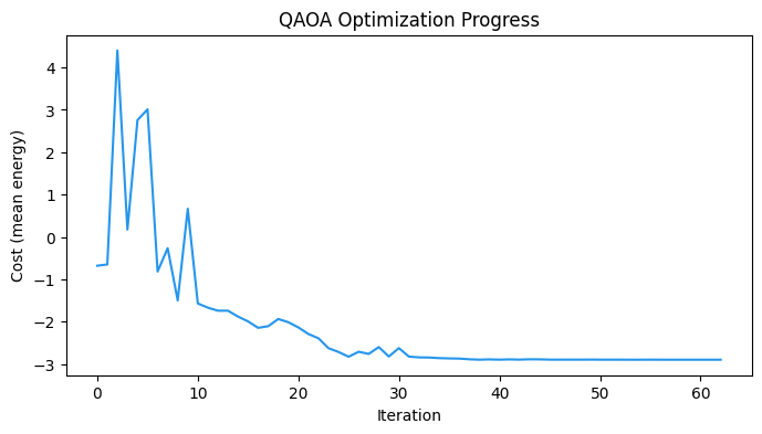

Decode and Analyze Results¶

We sample the circuit with the optimized parameters and interpret the measurement outcomes. decode_from_sampleresult returns samples already in the spin domain (+1 / -1), so we can count cut edges directly — no binary conversion needed.

gammas_opt = list(res.x[:p])
betas_opt = list(res.x[p:])

final_result = executable.sample(
    executor,
    shots=sample_shots,
    bindings={"gammas": gammas_opt, "betas": betas_opt},
).result()

decoded = spin_model.decode_from_sampleresult(final_result)

from collections import Counter

cut_distribution: Counter[int] = Counter()
best_qaoa_cut = 0
best_qaoa_sample = None

for sample, _energy, occ in zip(
    decoded.samples, decoded.energy, decoded.num_occurrences
):
    # sample is a dict {vertex_index: spin_value (+1 or -1)}
    spins = [sample[i] for i in range(num_nodes)]
    cut = sum(1 for i, j in G.edges() if spins[i] != spins[j])
    cut_distribution[cut] += occ
    if cut > best_qaoa_cut:
        best_qaoa_cut = cut
        best_qaoa_sample = spins

print(f"Best QAOA cut: {best_qaoa_cut}  (optimal: {best_cut})")
print(f"Best partition (spins): {best_qaoa_sample}")

Best QAOA cut: 5  (optimal: 5)
Best partition (spins): [1, -1, -1, 1, -1]

cuts = sorted(cut_distribution.keys())
counts = [cut_distribution[c] for c in cuts]

plt.figure(figsize=(8, 4))
plt.bar([str(c) for c in cuts], counts, color="#2696EB")
plt.xlabel("Cut size")
plt.ylabel("Frequency")
plt.title("Distribution of MaxCut Values from QAOA")
plt.show()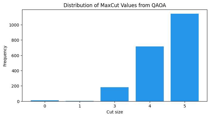

if best_qaoa_sample is not None:
    color_map = [
        "#FF6B6B" if best_qaoa_sample[i] == +1 else "#4ECDC4" for i in range(num_nodes)
    ]
    plt.figure(figsize=(5, 4))
    nx.draw(
        G,
        pos,
        with_labels=True,
        node_color=color_map,
        node_size=700,
        edgecolors="black",
    )
    plt.title(f"QAOA partition (cut = {best_qaoa_cut})")
    plt.show()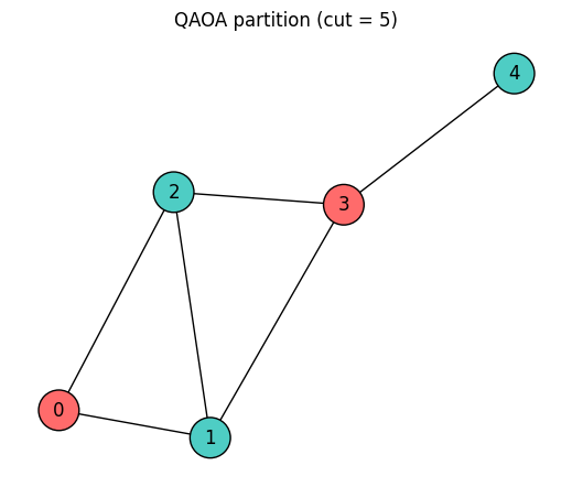

Using the Built-in `qaoa_state`¶

Everything we implemented above — superposition, cost layer, mixer layer, and the layered loop — is already provided by qamomile.circuit.algorithm.qaoa_state. It accepts exactly the same Ising coefficients (quad, linear) and variational parameters (gammas, betas).

Let’s build the same circuit using the built-in function to confirm that it implements the same structure. Each executor below is instantiated with the same seed_simulator=SEED. Under a fixed seed, identical circuits yield identical samples and therefore identical mean energies. With finite shots the per-circuit estimate still carries shot-noise — that does not vanish under seeding — so if the two printed mean energies do differ, it indicates that the manual and built-in routes did not emit bit-identical circuits (e.g., a gate ordering or compilation difference), not residual sampling noise.

from qamomile.circuit.algorithm import qaoa_state


@qmc.qkernel
def qaoa_builtin(
    p: qmc.UInt,
    quad: qmc.Dict[qmc.Tuple[qmc.UInt, qmc.UInt], qmc.Float],
    linear: qmc.Dict[qmc.UInt, qmc.Float],
    n: qmc.UInt,
    gammas: qmc.Vector[qmc.Float],
    betas: qmc.Vector[qmc.Float],
) -> qmc.Vector[qmc.Bit]:
    q = qaoa_state(p=p, quad=quad, linear=linear, n=n, gammas=gammas, betas=betas)
    return qmc.measure(q)

We transpile and sample with the same optimized parameters.

exe_builtin = transpiler.transpile(
    qaoa_builtin,
    bindings={
        "p": p,
        "quad": spin_model.quad,
        "linear": spin_model.linear,
        "n": num_nodes,
    },
    parameters=["gammas", "betas"],
)

executor_manual = transpiler.executor(backend=make_seeded_backend())
executor_builtin = transpiler.executor(backend=make_seeded_backend())

result_manual = executable.sample(
    executor_manual,
    shots=sample_shots,
    bindings={"gammas": gammas_opt, "betas": betas_opt},
).result()

result_builtin = exe_builtin.sample(
    executor_builtin,
    shots=sample_shots,
    bindings={"gammas": gammas_opt, "betas": betas_opt},
).result()

decoded_manual = spin_model.decode_from_sampleresult(result_manual)
decoded_builtin = spin_model.decode_from_sampleresult(result_builtin)
print(f"Manual   mean energy: {decoded_manual.energy_mean():.4f}")
print(f"Built-in mean energy: {decoded_builtin.energy_mean():.4f}")

Manual   mean energy: -2.8955
Built-in mean energy: -2.8955

Summary¶

In this tutorial we:

Defined a MaxCut problem and wrote it directly as an Ising Hamiltonian on spin variables — no QUBO / binary-variable detour.
Built the spin-domain BinaryModel with BinaryModel.from_ising.
Built every component of the QAOA circuit as a @qkernel — superposition, cost layer, mixer layer, and the full ansatz.
Ran a classical optimization loop and decoded the spin-domain results.
Verified that qamomile.circuit.algorithm.qaoa_state provides the same circuit with a single function call.

The same spin-first recipe applies to any Ising-like problem — spin-glass ground-state search, weighted MaxCut, Sherrington–Kirkpatrick model, and so on: plug the $h_i$ and $J_{ij}$ coefficients into BinaryModel.from_ising and reuse the circuit components above.

Next steps:

For problems that are naturally expressed with binary variables or that require constraints (penalty terms), see QAOA for Graph Partitioning, which uses the higher-level QAOAConverter together with JijModeling.