Quantum Selected Configuration Interaction (QSCI)

Tags: algorithm sample-based

QSCI is a hybrid quantum–classical algorithm that uses bitstrings sampled from a quantum state to build a small effective Hamiltonian and then diagonalizes it exactly on a classical computer. The advantage over plain VQE is that the result inherits a strict variational guarantee: even on noisy hardware,

E_{\mathrm{QSCI}} \;\geq\; E_{\mathrm{exact}}.

(1)

The four-step recipe introduced by Kanno et al. Kanno et al., 2023 is:

Prepare an input state $|\psi_{\mathrm{in}}\rangle$ on the quantum computer (typically a roughly optimised VQE state).
Measure $|\psi_{\mathrm{in}}\rangle$ in the computational basis many times.
Pick the top- $K$ most-frequent bitstrings as a discrete subspace $\{|s_i\rangle\}_{i=1}^{K}$ .
Build the effective Hamiltonian $H^{\mathrm{sub}}_{ij} = \langle s_i | H | s_j \rangle$ and diagonalize it classically.

This tutorial walks through the full flow on a four-qubit transverse- field Ising model. The quantum state preparation and sampling run on the QURI Parts backend (Qulacs simulator); the subspace construction and diagonalization use qamomile.linalg.solve_subspace, which internally calls the vectorised Z-basis routine subspace_hamiltonian (XOR / parity, no matrix products).

import os

import matplotlib.pyplot as plt
import numpy as np
from scipy.optimize import minimize

import qamomile.circuit as qmc
import qamomile.observable as qm_o
from qamomile.circuit.algorithm.basic import cx_entangling_layer, ry_layer
from qamomile.linalg import solve_subspace
from qamomile.quri_parts import QuriPartsExecutor, QuriPartsTranspiler

docs_test_mode = os.environ.get("QAMOMILE_DOCS_TEST") == "1"

A small test Hamiltonian¶

We use the four-qubit transverse-field Ising model on an open chain:

H \;=\; -J \sum_{i=0}^{n-2} Z_i Z_{i+1} \;-\; h \sum_{i=0}^{n-1} X_i, \quad J = 1,\; h = 0.7.

(2)

The 16-dimensional Hilbert space is small enough that we can compute the exact ground-state energy directly with NumPy and use it as the QSCI reference.

n_qubits = 4
J = 1.0
h_field = 0.7

H = qm_o.Hamiltonian(num_qubits=n_qubits)
for i in range(n_qubits - 1):
    H += qm_o.Z(i) * qm_o.Z(i + 1) * (-J)
for i in range(n_qubits):
    H += qm_o.X(i) * (-h_field)

exact_eigvals = np.linalg.eigvalsh(H.to_numpy())
E_exact = float(exact_eigvals[0])
print(f"Exact ground state energy: {E_exact:.6f}")

Exact ground state energy: -3.872983

Hardware-efficient ansatz¶

A simple alternating-layer ansatz: each layer applies $R_y$ to every qubit followed by a linear chain of CX gates, plus a final $R_y$ layer. We define three helper kernels:

ansatz_state builds the $|\psi(\theta)\rangle$ qubit register;
ansatz_energy returns $\langle\psi|H|\psi\rangle$ for VQE;
ansatz_measure measures the state in the computational basis for QSCI sampling.

@qmc.qkernel
def ansatz_state(
    n: qmc.UInt,
    reps: qmc.UInt,
    thetas: qmc.Vector[qmc.Float],
) -> qmc.Vector[qmc.Qubit]:
    q = qmc.qubit_array(n, name="q")
    for r in qmc.range(reps):
        q = ry_layer(q, thetas, r * n)
        q = cx_entangling_layer(q)
    final_base = reps * n
    q = ry_layer(q, thetas, final_base)
    return q


@qmc.qkernel
def ansatz_energy(
    n: qmc.UInt,
    reps: qmc.UInt,
    thetas: qmc.Vector[qmc.Float],
    H: qmc.Observable,
) -> qmc.Float:
    q = ansatz_state(n, reps, thetas)
    return qmc.expval(q, H)


@qmc.qkernel
def ansatz_measure(
    n: qmc.UInt,
    reps: qmc.UInt,
    thetas: qmc.Vector[qmc.Float],
) -> qmc.Vector[qmc.Bit]:
    q = ansatz_state(n, reps, thetas)
    return qmc.measure(q)

Compile both kernels with the QURI Parts backend¶

transpiler = QuriPartsTranspiler()
executor = QuriPartsExecutor()

reps = 2
n_params = (reps + 1) * n_qubits

energy_exec = transpiler.transpile(
    ansatz_energy,
    bindings={"n": n_qubits, "reps": reps, "H": H},
    parameters=["thetas"],
)
sample_exec = transpiler.transpile(
    ansatz_measure,
    bindings={"n": n_qubits, "reps": reps},
    parameters=["thetas"],
)

Step 1: Prepare $|\psi_{\mathrm{in}}\rangle$ via a quick VQE¶

QSCI is robust to a poorly optimised input state — even random parameters give a meaningful subspace — but a short VQE run concentrates the sampling distribution on the bitstrings that dominate the true ground state, making the subspace much more informative for a given $K$ . We run only a handful of COBYLA iterations.

def cost_fn(params: np.ndarray) -> float:
    return energy_exec.run(
        executor, bindings={"thetas": list(params)}
    ).result()


rng = np.random.default_rng(0)
init_params = rng.uniform(0, 2 * np.pi, n_params)

maxiter = max(n_params + 2, 5 if docs_test_mode else 80)
result = minimize(
    cost_fn,
    init_params,
    method="COBYLA",
    options={"maxiter": maxiter, "rhobeg": 0.5},
)
opt_params = result.x
print(f"VQE energy = {result.fun:+.6f}   (gap to E_exact: {result.fun - E_exact:.4e})")

VQE energy = -3.719549   (gap to E_exact: 1.5343e-01)

Step 2: Sample bitstrings in the Z basis¶

Each sample is a tuple (b_0, ..., b_{n-1}) whose $q$ -th entry is the Z-eigenvalue index of qubit $q$ — exactly the format subspace_hamiltonian expects.

shots = 500 if docs_test_mode else 4000
sample_results = (
    sample_exec.sample(
        executor, bindings={"thetas": list(opt_params)}, shots=shots
    )
    .result()
    .results
)
sample_results.sort(key=lambda bc: bc[1], reverse=True)
print(f"Distinct bitstrings sampled: {len(sample_results)}")
for bits, c in sample_results[:5]:
    print(f"  {bits}  count={c}")

Distinct bitstrings sampled: 14
  (1, 1, 1, 1)  count=2848
  (1, 1, 1, 0)  count=411
  (0, 1, 1, 1)  count=316
  (1, 0, 1, 1)  count=114
  (1, 1, 0, 1)  count=107

Step 3 + 4: Build the QSCI subspace and diagonalize¶

For each subspace size $K$ we feed the $K$ most-frequent bitstrings to solve_subspace, which builds $H^{\mathrm{sub}}_{ij} = \langle s_i|H|s_j\rangle$ via a vectorised XOR / parity routine and runs numpy.linalg.eigh. The lowest returned eigenvalue is the QSCI energy estimate, and the variational principle guarantees $E_{\mathrm{QSCI}}(K) \geq E_{\mathrm{exact}}$ for every $K$ .

unique_bitstrings = [bits for bits, _ in sample_results]
K_max = len(unique_bitstrings)
ks = sorted({k for k in (1, 2, 4, 8, 16, K_max) if k <= K_max})

energies = [
    float(solve_subspace(unique_bitstrings[:K], H)[0][0]) for K in ks
]

for K, E in zip(ks, energies):
    print(f"K = {K:3d}   E_QSCI = {E:+.6f}   gap = {E - E_exact:+.3e}")

assert all(E >= E_exact - 1e-9 for E in energies), "variational bound violated"

K =   1   E_QSCI = -3.000000   gap = +8.730e-01
K =   2   E_QSCI = -3.220656   gap = +6.523e-01
K =   4   E_QSCI = -3.500753   gap = +3.722e-01
K =   8   E_QSCI = -3.682559   gap = +1.904e-01
K =  14   E_QSCI = -3.750479   gap = +1.225e-01

fig, ax = plt.subplots(figsize=(6, 4))
ax.plot(ks, energies, "-o", label=r"$E_{\mathrm{QSCI}}$")
ax.axhline(E_exact, color="black", linestyle="--", label=r"$E_{\mathrm{exact}}$")
ax.set_xlabel("Subspace size $K$")
ax.set_ylabel("Energy")
ax.set_title("QSCI convergence — 4-qubit TFIM ($J{=}1,\\;h{=}0.7$)")
ax.legend()
ax.grid(True, alpha=0.3)
plt.tight_layout()
plt.show()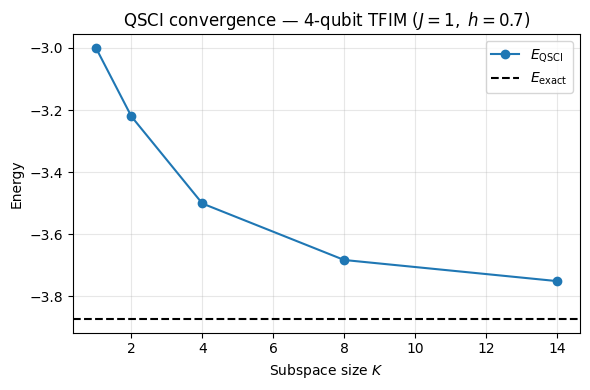

Notes¶

The Z-basis fast path (subspace_hamiltonian) used inside solve_subspace requires no matrix multiplication: each Pauli term contributes a single XOR mask and parity sign, vectorised across all $K^2$ sample pairs.
Duplicate sampled bitstrings drop out of the unique-bitstring list above; the resulting subspace is well-conditioned and solve_subspace returns an ordinary Hermitian eigendecomposition.

References¶

Kanno, K., Kohda, M., Imai, R., Koh, S., Mitarai, K., Mizukami, W., & Nakagawa, Y. O. (2023). Quantum-Selected Configuration Interaction: classical diagonalization of Hamiltonians in subspaces selected by quantum computers. arXiv. 10.48550/ARXIV.2302.11320