QAOA for MaxCut: Building the Circuit from Scratch

This tutorial walks through the Quantum Approximate Optimization Algorithm (QAOA) pipeline step by step, using Qamomile’s low-level circuit primitives. Rather than using the high-level QAOAConverter, we will:

Define a MaxCut problem for a small graph.
Formulate it as a QUBO, then convert to an Ising model.
Write the QAOA circuit step by step using @qkernel.
Optimize variational parameters with a classical optimizer.
Decode and visualize the results.

At the end, we show that qamomile.circuit.algorithm.qaoa_state provides the same circuit in a single function call.

# Install the latest Qamomile through pip!
# !pip install qamomile

What is MaxCut?¶

Given an undirected graph $G = (V, E)$ , the MaxCut problem asks us to partition the vertices into two sets $S$ and $\bar{S}$ so that the number of edges between the two sets is maximized:

\text{MaxCut}(x) = \sum_{(i,j) \in E} x_i (1 - x_j) + x_j (1 - x_i)

(1)

where $x_i \in \{0, 1\}$ indicates which set vertex $i$ belongs to.

Create the Graph¶

We use a small 5-node graph with 6 edges. This is large enough to be non-trivial, yet small enough to brute-force for comparison.

import matplotlib.pyplot as plt
import networkx as nx

G = nx.Graph()
G.add_edges_from([(0, 1), (0, 2), (1, 2), (1, 3), (2, 3), (3, 4)])
num_nodes = G.number_of_nodes()

pos = nx.spring_layout(G, seed=42)
plt.figure(figsize=(5, 4))
nx.draw(
    G,
    pos,
    with_labels=True,
    node_color="white",
    node_size=700,
    edgecolors="black",
)
plt.title(f"Graph: {num_nodes} nodes, {G.number_of_edges()} edges")
plt.show()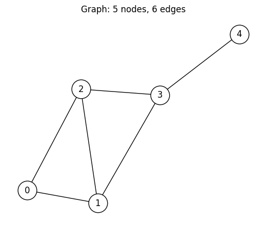

QUBO Formulation¶

To minimize with QAOA, we negate the MaxCut objective:

\min_x \sum_{(i,j) \in E} \bigl(2 x_i x_j - x_i - x_j \bigr)

(2)

This maps to a QUBO dictionary where each edge $(i, j)$ contributes:

$Q_{ii} \mathrel{-}= 1$ , $Q_{jj} \mathrel{-}= 1$ (diagonal)
$Q_{ij} \mathrel{+}= 2$ (off-diagonal)

from qamomile.optimization.binary_model import BinaryModel, VarType

# Build QUBO dictionary from graph edges
qubo: dict[tuple[int, int], float] = {}
for i, j in G.edges():
    qubo[(i, i)] = qubo.get((i, i), 0.0) - 1.0
    qubo[(j, j)] = qubo.get((j, j), 0.0) - 1.0
    qubo[(i, j)] = qubo.get((i, j), 0.0) + 2.0

print("QUBO coefficients:")
for key, val in sorted(qubo.items()):
    print(f"  {key}: {val}")

model = BinaryModel.from_qubo(qubo)
print(f"\nNumber of variables: {model.num_bits}")
print(f"Variable type: {model.vartype}")

QUBO coefficients:
  (0, 0): -2.0
  (0, 1): 2.0
  (0, 2): 2.0
  (1, 1): -3.0
  (1, 2): 2.0
  (1, 3): 2.0
  (2, 2): -3.0
  (2, 3): 2.0
  (3, 3): -3.0
  (3, 4): 2.0
  (4, 4): -1.0

Number of variables: 5
Variable type: BINARY

Note: BinaryModel also provides from_ising() and from_hubo() constructors for other input formats. Use change_vartype() to convert between binary and spin representations.

From QUBO to Ising Model¶

QAOA operates in the spin domain ( $s_i \in \{+1, -1\}$ ), not the binary domain ( $x_i \in \{0, 1\}$ ). The conversion is:

x_i = \frac{1 - s_i}{2}

(3)

This matches the quantum convention $Z|0\rangle = |0\rangle$ , $Z|1\rangle = -|1\rangle$ , so binary 0 maps to spin +1 and binary 1 maps to spin -1.

Substituting into the QUBO yields an Ising Hamiltonian:

H = \sum_i h_i \, s_i + \sum_{i < j} J_{ij} \, s_i \, s_j + \text{const}

(4)

spin_model = model.change_vartype(VarType.SPIN).normalize_by_abs_max()

print(f"Variable type: {spin_model.vartype}")
print(f"Linear terms (h_i):     {spin_model.linear}")
print(f"Quadratic terms (J_ij): {spin_model.quad}")
print(f"Constant:               {spin_model.constant}")

Variable type: SPIN
Linear terms (h_i):     {}
Quadratic terms (J_ij): {(0, 1): 1.0, (0, 2): 1.0, (1, 2): 1.0, (1, 3): 1.0, (2, 3): 1.0, (3, 4): 1.0}
Constant:               -6.0

Exact Solution (Brute Force)¶

Before running QAOA, let’s find the optimal solution by trying all $2^n = 32$ partitions. This gives us a ground truth to compare against.

import itertools

best_cut = 0
optimal_partitions: list[tuple[int, ...]] = []

for bits in itertools.product([0, 1], repeat=num_nodes):
    cut = sum(1 for i, j in G.edges() if bits[i] != bits[j])
    if cut > best_cut:
        best_cut = cut
        optimal_partitions = [bits]
    elif cut == best_cut:
        optimal_partitions.append(bits)

print(f"Optimal MaxCut value: {best_cut}")
print(f"Number of optimal partitions: {len(optimal_partitions)}")
for part in optimal_partitions:
    print(f"  {part}")

Optimal MaxCut value: 5
Number of optimal partitions: 2
  (0, 1, 1, 0, 1)
  (1, 0, 0, 1, 0)

QAOA Circuit: The Idea¶

The QAOA ansatz prepares a parameterized quantum state:

|\boldsymbol{\gamma}, \boldsymbol{\beta}\rangle = \prod_{l=1}^{p} e^{-i \beta_l H_M} \, e^{-i \gamma_l H_C} \; |{+}\rangle^{\otimes n}

(5)

where:

$|{+}\rangle^{\otimes n}$ : uniform superposition (Hadamard on every qubit)
$e^{-i \gamma H_C}$ : cost unitary — for an Ising cost, this decomposes into $\text{RZZ}$ and $\text{RZ}$ gates (see Steps 2–3 for the gate convention details)
$e^{-i \beta H_M}$ : mixer unitary — with $H_M = \sum_i X_i$ , this becomes $\text{RX}(2\beta)$ on every qubit
$p$ : number of layers (depth of the ansatz)

We will now build each component as a @qkernel.

Step 1: Uniform Superposition¶

Apply a Hadamard gate to every qubit to start from the equal superposition state $|{+}\rangle^{\otimes n}$ .

import qamomile.circuit as qmc


@qmc.qkernel
def superposition(n: qmc.UInt) -> qmc.Vector[qmc.Qubit]:
    q = qmc.qubit_array(n, name="q")
    for i in qmc.range(n):
        q[i] = qmc.h(q[i])
    return q

Step 2: Cost Layer¶

Apply the cost unitary $e^{-i \gamma H_C}$ .

Qamomile’s rotation gates include a $1/2$ factor: $\text{RZ}(\theta) = e^{-i \theta Z / 2}$ and $\text{RZZ}(\theta) = e^{-i \theta Z \otimes Z / 2}$ . To match $e^{-i \gamma H_C}$ exactly one would pass $2 J_{ij} \gamma$ as the angle. However, since $\gamma$ is a variational parameter that the classical optimizer tunes freely, this constant factor is simply absorbed into the optimal $\gamma$ values. We therefore pass $J_{ij} \cdot \gamma$ (and $h_i \cdot \gamma$ ) directly:

@qmc.qkernel
def cost_layer(
    quad: qmc.Dict[qmc.Tuple[qmc.UInt, qmc.UInt], qmc.Float],
    linear: qmc.Dict[qmc.UInt, qmc.Float],
    q: qmc.Vector[qmc.Qubit],
    gamma: qmc.Float,
) -> qmc.Vector[qmc.Qubit]:
    for (i, j), Jij in quad.items():
        q[i], q[j] = qmc.rzz(q[i], q[j], angle=Jij * gamma)
    for i, hi in linear.items():
        q[i] = qmc.rz(q[i], angle=hi * gamma)
    return q

Step 3: Mixer Layer¶

Apply the mixer unitary $e^{-i \beta H_M}$ where $H_M = \sum_i X_i$ . Since $\text{RX}(\theta) = e^{-i \theta X / 2}$ , we need $\theta = 2\beta$ to implement $e^{-i \beta X_i}$ on each qubit.

@qmc.qkernel
def mixer_layer(
    q: qmc.Vector[qmc.Qubit],
    beta: qmc.Float,
) -> qmc.Vector[qmc.Qubit]:
    n = q.shape[0]
    for i in qmc.range(n):
        q[i] = qmc.rx(q[i], angle=2.0 * beta)
    return q

Step 4: Full QAOA Ansatz¶

Compose the three pieces: superposition, then $p$ rounds of cost + mixer, and finally measurement.

@qmc.qkernel
def qaoa_ansatz(
    p: qmc.UInt,
    quad: qmc.Dict[qmc.Tuple[qmc.UInt, qmc.UInt], qmc.Float],
    linear: qmc.Dict[qmc.UInt, qmc.Float],
    n: qmc.UInt,
    gammas: qmc.Vector[qmc.Float],
    betas: qmc.Vector[qmc.Float],
) -> qmc.Vector[qmc.Bit]:
    q = superposition(n)
    for layer in qmc.range(p):
        q = cost_layer(quad, linear, q, gammas[layer])
        q = mixer_layer(q, betas[layer])
    return qmc.measure(q)

Transpile and Optimize¶

We transpile the kernel, binding the problem structure (graph coefficients, number of qubits, number of layers) while keeping gammas and betas as runtime parameters that the optimizer will tune.

from qamomile.qiskit import QiskitTranspiler

transpiler = QiskitTranspiler()
p = 3  # number of QAOA layers

executable = transpiler.transpile(
    qaoa_ansatz,
    bindings={
        "p": p,
        "quad": spin_model.quad,
        "linear": spin_model.linear,
        "n": num_nodes,
    },
    parameters=["gammas", "betas"],
)

We use scipy.optimize.minimize with the COBYLA method. At each iteration, the optimizer samples the circuit and evaluates the mean energy.

import numpy as np
from qiskit_aer import AerSimulator
from scipy.optimize import minimize

executor = transpiler.executor(backend=AerSimulator(seed_simulator=7))
cost_history: list[float] = []


def cost_fn(params):
    gammas = list(params[:p])
    betas = list(params[p:])
    result = executable.sample(
        executor,
        shots=2048,
        bindings={"gammas": gammas, "betas": betas},
    ).result()
    decoded = spin_model.decode_from_sampleresult(result)
    energy = decoded.energy_mean()
    cost_history.append(energy)
    return energy


rng = np.random.default_rng(42)
initial_params = rng.uniform(-np.pi / 2, np.pi / 2, 2 * p)

res = minimize(cost_fn, initial_params, method="COBYLA", options={"maxiter": 500})

print(f"Optimized cost: {res.fun:.4f}")
print(f"Optimal params: {[round(v, 4) for v in res.x]}")

Optimized cost: -8.8896
Optimal params: [np.float64(0.8252), np.float64(-0.2989), np.float64(1.4505), np.float64(0.4523), np.float64(-0.8443), np.float64(2.9848)]

plt.figure(figsize=(8, 4))
plt.plot(cost_history, color="#2696EB")
plt.xlabel("Iteration")
plt.ylabel("Cost (mean energy)")
plt.title("QAOA Optimization Progress")
plt.show()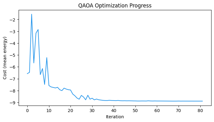

Decode and Analyze Results¶

We sample the circuit with the optimized parameters and interpret the measurement outcomes. For MaxCut every bitstring is a valid partition, so there is no feasibility check needed — we simply count the cut edges for each sample.

gammas_opt = list(res.x[:p])
betas_opt = list(res.x[p:])

final_result = executable.sample(
    executor,
    shots=2048,
    bindings={"gammas": gammas_opt, "betas": betas_opt},
).result()

decoded = spin_model.decode_from_sampleresult(final_result)

from collections import Counter

cut_distribution: Counter[int] = Counter()
best_qaoa_cut = 0
best_qaoa_sample = None

for sample, energy, occ in zip(
    decoded.samples, decoded.energy, decoded.num_occurrences
):
    # Convert spin (+1/-1) back to binary (0/1): x = (1 - s) / 2
    binary = {idx: (1 - s) // 2 for idx, s in sample.items()}
    bits = [binary[i] for i in range(num_nodes)]
    cut = sum(1 for i, j in G.edges() if bits[i] != bits[j])
    cut_distribution[cut] += occ
    if cut > best_qaoa_cut:
        best_qaoa_cut = cut
        best_qaoa_sample = bits

print(f"Best QAOA cut: {best_qaoa_cut}  (optimal: {best_cut})")
print(f"Best partition: {best_qaoa_sample}")

Best QAOA cut: 5  (optimal: 5)
Best partition: [0, 1, 1, 0, 1]

cuts = sorted(cut_distribution.keys())
counts = [cut_distribution[c] for c in cuts]

plt.figure(figsize=(8, 4))
plt.bar([str(c) for c in cuts], counts, color="#2696EB")
plt.xlabel("Cut size")
plt.ylabel("Frequency")
plt.title("Distribution of MaxCut Values from QAOA")
plt.show()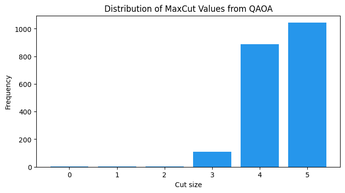

if best_qaoa_sample is not None:
    color_map = [
        "#FF6B6B" if best_qaoa_sample[i] == 1 else "#4ECDC4" for i in range(num_nodes)
    ]
    plt.figure(figsize=(5, 4))
    nx.draw(
        G,
        pos,
        with_labels=True,
        node_color=color_map,
        node_size=700,
        edgecolors="black",
    )
    plt.title(f"QAOA partition (cut = {best_qaoa_cut})")
    plt.show()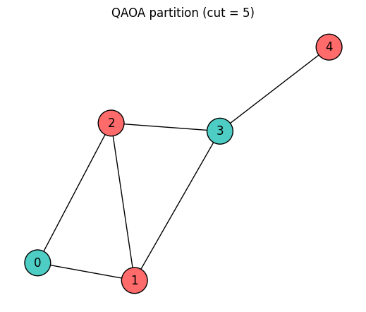

Using the Built-in `qaoa_state`¶

Everything we implemented above — superposition, cost layer, mixer layer, and the layered loop — is already provided by qamomile.circuit.algorithm.qaoa_state. It accepts exactly the same Ising coefficients (quad, linear) and variational parameters (gammas, betas).

Let’s build the same circuit using the built-in function to confirm that it implements the same structure. By using a seeded simulator, we can verify that both circuits produce identical results.

from qamomile.circuit.algorithm import qaoa_state


@qmc.qkernel
def qaoa_builtin(
    p: qmc.UInt,
    quad: qmc.Dict[qmc.Tuple[qmc.UInt, qmc.UInt], qmc.Float],
    linear: qmc.Dict[qmc.UInt, qmc.Float],
    n: qmc.UInt,
    gammas: qmc.Vector[qmc.Float],
    betas: qmc.Vector[qmc.Float],
) -> qmc.Vector[qmc.Bit]:
    q = qaoa_state(p=p, quad=quad, linear=linear, n=n, gammas=gammas, betas=betas)
    return qmc.measure(q)

We transpile and sample with the same optimized parameters. Using a seeded AerSimulator gives deterministic results for identical circuits.

from qiskit_aer import AerSimulator

exe_builtin = transpiler.transpile(
    qaoa_builtin,
    bindings={
        "p": p,
        "quad": spin_model.quad,
        "linear": spin_model.linear,
        "n": num_nodes,
    },
    parameters=["gammas", "betas"],
)

seeded_executor_manual = transpiler.executor(
    backend=AerSimulator(seed_simulator=0),
)
seeded_executor_builtin = transpiler.executor(
    backend=AerSimulator(seed_simulator=0),
)

result_manual = executable.sample(
    seeded_executor_manual,
    shots=2048,
    bindings={"gammas": gammas_opt, "betas": betas_opt},
).result()

result_builtin = exe_builtin.sample(
    seeded_executor_builtin,
    shots=2048,
    bindings={"gammas": gammas_opt, "betas": betas_opt},
).result()

decoded_manual = spin_model.decode_from_sampleresult(result_manual)
decoded_builtin = spin_model.decode_from_sampleresult(result_builtin)
print(f"Manual   mean energy: {decoded_manual.energy_mean():.4f}")
print(f"Built-in mean energy: {decoded_builtin.energy_mean():.4f}")

Manual   mean energy: -8.8838
Built-in mean energy: -8.8838

Summary¶

In this tutorial we:

Defined a MaxCut problem and built its QUBO formulation from a NetworkX graph.
Converted the QUBO to an Ising model using BinaryModel.
Built every component of the QAOA circuit as a @qkernel — superposition, cost layer, mixer layer, and the full ansatz.
Ran a classical optimization loop and decoded the results.
Verified that qamomile.circuit.algorithm.qaoa_state provides the same circuit with a single function call.

Next steps:

For constrained optimization problems (where penalty terms are needed), see QAOA for Graph Partitioning which uses the higher-level QAOAConverter together with JijModeling.