Quantum Phase Estimation (QPE)

Tags: algorithm primitive resource-estimation

Quantum Phase Estimation (QPE) estimates the eigenphase $\phi$ of a unitary matrix $U$ from an eigenstate $|\psi\rangle$ satisfying $U|\psi\rangle = e^{2\pi i \phi}|\psi\rangle$ . It is a central primitive in Shor’s algorithm and other algorithms that use phases encoded by the eigenvalues of unitary matrices Kitaev, 1995Cleve et al., 1998.

This notebook implements the QPE procedure as a Qamomile qkernel and compares it with the built-in qmc.qpe function. It then explores the relationship between the number of counting qubits, phase-estimation precision, and gate count.

# Install the latest Qamomile and the extras used by this notebook.
# !pip install "qamomile[qiskit,visualization]"

# Import numerical, plotting, simulator, and Qamomile utilities.
import math
import os

import matplotlib.pyplot as plt
import numpy as np
from qiskit_aer import AerSimulator

import qamomile.circuit as qmc
from qamomile.qiskit import QiskitTranspiler

transpiler = QiskitTranspiler()

Background: Phase Kickback and Quantum Fourier Transform¶

QPE combines two ideas: phase kickback from controlled unitaries Cleve et al., 1998 and the Quantum Fourier Transform Coppersmith, 2002.

Phase Kickback¶

Phase kickback is the mechanism by which, when a controlled- $U$ gate is applied to an eigenstate $|\psi\rangle$ of a unitary matrix $U$ , the eigenphase of $U$ appears as a relative phase on the control qubit. Suppose

U|\psi\rangle = e^{2\pi i\phi}|\psi\rangle.

(1)

Prepare one control qubit in a superposition and the target quantum state in $|\psi\rangle$ :

\frac{|0\rangle + |1\rangle}{\sqrt{2}}|\psi\rangle.

(2)

A controlled- $U$ gate applies $U$ only to the component in which the control qubit is $|1\rangle$ . Because $|\psi\rangle$ is an eigenstate of $U$ , the eigenphase appears on that component:

\frac{|0\rangle|\psi\rangle + |1\rangle U|\psi\rangle}{\sqrt{2}} = \frac{|0\rangle + e^{2\pi i\phi}|1\rangle}{\sqrt{2}}|\psi\rangle.

(3)

This transformation leaves the target quantum state in $|\psi\rangle$ and encodes the eigenphase in the relative phase of the control qubit. QPE deliberately uses this mechanism with multiple control qubits. The Algorithm section explains the encoding in detail.

Quantum Fourier Transform¶

The Quantum Fourier Transform (QFT) maps a computational-basis state to a superposition whose relative phases encode that state’s value. On $M=2^m$ basis states, the QFT is defined as

\mathrm{QFT}_M|x\rangle = \frac{1}{\sqrt{M}} \sum_{y=0}^{M-1} e^{2\pi i xy/M}|y\rangle.

(4)

It maps an integer $x$ to a regular phase pattern across the computational basis. We refer to a state that stores a value in these relative phases as a Fourier-encoded state. For an application in Qamomile, see the multidimensional QFT example. The inverse QFT $\mathrm{QFT}_M^{-1}$ performs the reverse operation. If $\phi=a/M$ is exactly representable with $m$ bits, then the controlled powers $U^{2^0}, U^{2^1}, \ldots, U^{2^{m-1}}$ prepare the counting register as

\frac{1}{\sqrt{M}}\sum_{k=0}^{M-1} e^{2\pi i a k/M}|k\rangle = \mathrm{QFT}_M|a\rangle.

(5)

Applying $\mathrm{QFT}_M^{-1}$ then returns $|a\rangle$ . The important point is that the inverse QFT turns phase information into a computational-basis bit string.

\underbrace{ \frac{1}{\sqrt{M}} \begin{pmatrix} 1 \\ e^{2\pi i a/M} \\ \vdots \\ e^{2\pi i a(M-1)/M} \end{pmatrix} }_{\text{vector of phase values}} \xrightarrow{\mathrm{QFT}_M^{-1}} \underbrace{|a\rangle = |a_{m-1}\cdots a_0\rangle}_{\text{computational-basis bit string}}.

(6)

Algorithm¶

QPE uses two groups of qubits: $m$ counting qubits that read out the phase and target qubits that hold an eigenstate $|\psi\rangle$ of $U$ . The counting qubits are auxiliary qubits used to represent the phase as an $m$ -bit binary fraction. Suppose $U|\psi\rangle=e^{2\pi i\phi}|\psi\rangle$ . The counting qubits start in $|0\rangle^{\otimes m}$ , and we write $M=2^m$ .

Step 1: Put the counting qubits in superposition¶

Apply Hadamard gates to the counting qubits. This creates a uniform superposition over the $M$ possible values.

|\Psi_1\rangle = H^{\otimes m}|0\rangle^{\otimes m}|\psi\rangle = \frac{1}{\sqrt{M}}\sum_{r=0}^{M-1}|r\rangle|\psi\rangle.

(7)

Step 2: Apply controlled- $U^{2^k}$ gates¶

Use each counting qubit $k$ as the control qubit for a controlled- $U^{2^k}$ gate. If $r=\sum_{k=0}^{m-1} r_k2^k$ , the target eigenstate picks up the phase $e^{2\pi i\phi r}$ :

|\Psi_2\rangle = \frac{1}{\sqrt{M}}\sum_{r=0}^{M-1} e^{2\pi i \phi r}|r\rangle|\psi\rangle.

(8)

Step 3: Convert phase information into a bit string with inverse QFT¶

If $\phi=a/M$ is exactly representable, the counting register is $\mathrm{QFT}_M|a\rangle$ . Applying the inverse QFT returns $|a\rangle$ .

|\Psi_2\rangle = \left( \frac{1}{\sqrt{M}}\sum_{r=0}^{M-1} e^{2\pi i ar/M}|r\rangle \right)|\psi\rangle = \mathrm{QFT}_M|a\rangle|\psi\rangle,

(9)

|\Psi_3\rangle = \mathrm{QFT}_M^{-1}\mathrm{QFT}_M|a\rangle|\psi\rangle = |a\rangle|\psi\rangle.

(10)

Step 4: Measure the bit string and decode the phase¶

Measure the counting qubits. In the exact case, the measurement returns $a$ , and decoding this bit string gives the phase estimate

\tilde{\phi} = \frac{a}{M}.

(11)

If $\phi$ is not exactly representable with $m$ bits, the distribution concentrates around the closest $m$ -bit approximations. Increasing $m$ reduces the spacing between representable phases to $1/2^m$ , allowing the estimate to approach the true eigenphase.

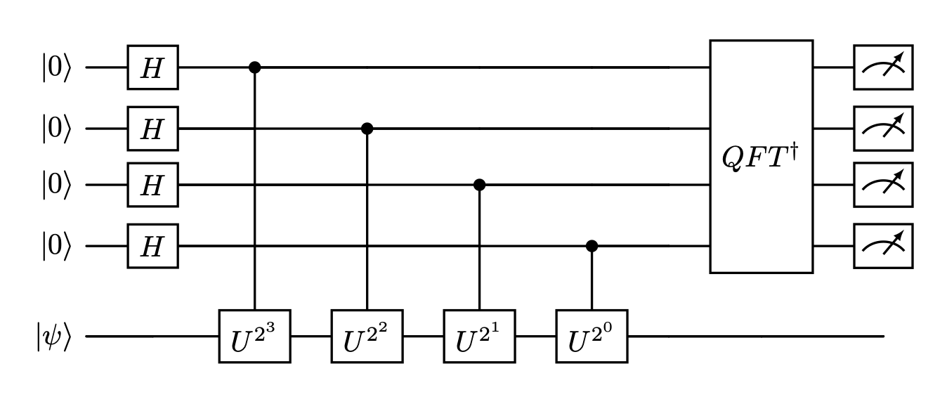
Quantum phase estimation circuit with a counting register, controlled powers of U, inverse QFT, and measurement. — Schematic QPE circuit. The counting register controls the powers of $U$ , and the inverse QFT converts the accumulated phase pattern into measured bits.

Implementation with Qamomile¶

We use a diagonal 4x4 unitary matrix:

U = \begin{pmatrix} 1 & 0 & 0 & 0 \\ 0 & e^{i\theta_{01}} & 0 & 0 \\ 0 & 0 & e^{i\theta_{10}} & 0 \\ 0 & 0 & 0 & e^{i\theta_{11}} \end{pmatrix}.

(14)

Every computational-basis state is an eigenstate of this matrix. We prepare the target state $|01\rangle$ and set the phase to estimate, $\theta_{01} / 2\pi$ , to 0.6. Because 0.6 is not exactly representable on a finite binary fraction, increasing the number of counting qubits visibly improves the approximation.

# Set the sampling settings and target eigenstate.
docs_test_mode = os.environ.get("QAMOMILE_DOCS_TEST") == "1"
SHOTS = 512 if docs_test_mode else 4096
SAMPLER_SEED = 42

# Set the phases of the diagonal unitary matrix and the target phase.
TARGET_PHASE_FRACTION = 0.6
phase_fractions = np.array([0.0, TARGET_PHASE_FRACTION, 0.23, 0.81])
phase_angles = 2 * math.pi * phase_fractions

# Convert the phase fractions to a unitary matrix and check unitarity.
unitary = np.diag(np.exp(1j * phase_angles))
assert np.allclose(unitary.conj().T @ unitary, np.eye(4))

# Store the concrete phase parameters used by the qkernel.
PHI_01 = float(phase_angles[1])
PHI_10 = float(phase_angles[2])
PHI_11 = float(phase_angles[3])

# Print the problem instance for reference.
print("phase fractions:", np.round(phase_fractions, 6))
print("target phase fraction:", f"{TARGET_PHASE_FRACTION:.8f}")
print("U =")
print(np.round(unitary, 3))
assert 0.0 <= TARGET_PHASE_FRACTION < 1.0

phase fractions: [0.   0.6  0.23 0.81]
target phase fraction: 0.60000000
U =
[[ 1.   +0.j     0.   +0.j     0.   +0.j     0.   +0.j   ]
 [ 0.   +0.j    -0.809-0.588j  0.   +0.j     0.   +0.j   ]
 [ 0.   +0.j     0.   +0.j     0.125+0.992j  0.   +0.j   ]
 [ 0.   +0.j     0.   +0.j     0.   +0.j     0.368-0.93j ]]

From-Scratch Implementation¶

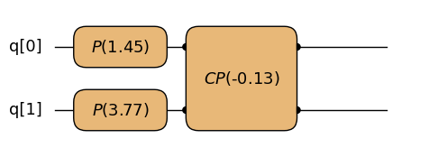
First, we define the 4x4 unitary matrix whose phase we want to estimate. The diagonal_4x4 qkernel implements this matrix directly. The phase gate $P(\theta)$ multiplies the $|1\rangle$ component of a qubit by $e^{i\theta}$ ; Qamomile expresses this gate as qmc.p(q, theta). Applying qmc.p(q[0], phi10) therefore gives every basis state whose first target bit is 1 the phase $e^{i\theta_{10}}$ , and qmc.p(q[1], phi01) gives every basis state whose second target bit is 1 the phase $e^{i\theta_{01}}$ . At that point $|11\rangle$ has accumulated $e^{i(\theta_{10}+\theta_{01})}$ , so the controlled phase gate adds only the correction

\theta_{11} - \theta_{10} - \theta_{01}

(15)

on $|11\rangle$ . The resulting diagonal is exactly $\operatorname{diag}(1, e^{i\theta_{01}}, e^{i\theta_{10}}, e^{i\theta_{11}})$ in the ordered basis $|00\rangle, |01\rangle, |10\rangle, |11\rangle$ .

# Implement the diagonal 4x4 unitary matrix with phase gates.
@qmc.qkernel
def diagonal_4x4(
    q: qmc.Vector[qmc.Qubit],
    phi01: qmc.Float,
    phi10: qmc.Float,
    phi11: qmc.Float,
) -> qmc.Vector[qmc.Qubit]:
    # Add phases controlled by each target bit.
    q[0] = qmc.p(q[0], phi10)
    q[1] = qmc.p(q[1], phi01)
    # Correct the |11> entry so the full diagonal matches the matrix.
    q[0], q[1] = qmc.cp(q[0], q[1], phi11 - phi10 - phi01)
    return q


# Draw the target unitary matrix with the concrete phase parameters.
diagonal_4x4.draw(
    q=2,
    phi01=PHI_01,
    phi10=PHI_10,
    phi11=PHI_11,
    fold_loops=False,
)

We now implement the four QPE steps using Qamomile’s basic operations. qmc.control(diagonal_4x4) constructs controlled- $U$ , and power=2**k applies controlled- $U^{2^k}$ . After the inverse QFT, the qubits are cast to a QFixed with no integer bits. qmc.measure measures those qubits and decodes the resulting bit string into a floating-point phase estimate.

# Implement QPE from basic operations.
controlled_diagonal_4x4 = qmc.control(diagonal_4x4)


@qmc.qkernel
def qpe_from_scratch(
    counting_bits: qmc.UInt,
    phi01: qmc.Float,
    phi10: qmc.Float,
    phi11: qmc.Float,
) -> qmc.Float:
    counting = qmc.qubit_array(counting_bits, name="counting")
    target = qmc.qubit_array(2, name="target")
    target[1] = qmc.x(target[1])

    for k in qmc.range(counting_bits):
        counting[k] = qmc.h(counting[k])
    for k in qmc.range(counting_bits):
        counting[k], target = controlled_diagonal_4x4(
            counting[k],
            target,
            phi01=phi01,
            phi10=phi10,
            phi11=phi11,
            power=2**k,
        )

    counting = qmc.iqft(counting)
    phase = qmc.cast(counting, qmc.QFixed, int_bits=0)
    return qmc.measure(phase)


# Draw the from-scratch implementation with three counting qubits.
qpe_from_scratch.draw(
    counting_bits=3,
    phi01=PHI_01,
    phi10=PHI_10,
    phi11=PHI_11,
    fold_loops=False,
)

Built-in Function: `qpe`¶

The qmc.qpe function combines the Hadamard gates, controlled- $U^{2^k}$ gates, inverse QFT, and cast to QFixed used in the from-scratch implementation. Passing the returned QFixed to qmc.measure measures the qubits and decodes the fixed-point bit string into a floating-point phase estimate.

# Implement the same QPE procedure with the built-in qpe function.
@qmc.qkernel
def qpe_with_stdlib(
    counting_bits: qmc.UInt,
    phi01: qmc.Float,
    phi10: qmc.Float,
    phi11: qmc.Float,
) -> qmc.Float:
    counting = qmc.qubit_array(counting_bits, name="counting")
    target = qmc.qubit_array(2, name="target")
    target[1] = qmc.x(target[1])

    phase = qmc.qpe(
        target,
        counting,
        diagonal_4x4,
        phi01=phi01,
        phi10=phi10,
        phi11=phi11,
    )
    return qmc.measure(phase)


# Draw the built-in implementation with three counting qubits.
qpe_with_stdlib.draw(
    counting_bits=3,
    phi01=PHI_01,
    phi10=PHI_10,
    phi11=PHI_11,
    fold_loops=False,
)

Execution Result¶

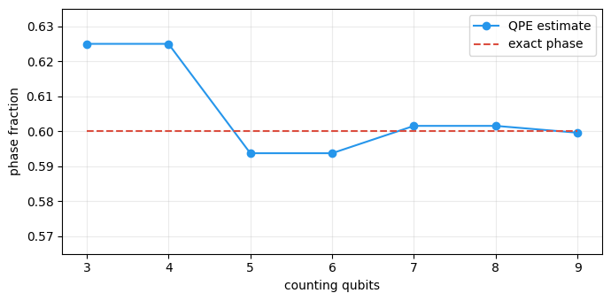
The target phase 0.6 cannot be represented exactly with only a few bits, so QPE returns a distribution over nearby $m$ -bit approximations. We vary the number of counting qubits from 3 to 9 and compare the estimate produced by the built-in qpe function with the exact phase.

# Bind the phases of the diagonal unitary matrix at transpile time.
phase_bindings = {"phi01": PHI_01, "phi10": PHI_10, "phi11": PHI_11}


# Compute cyclic distance between two phase fractions.
def phase_distance(a: float, b: float) -> float:
    raw_distance = abs(a - b)
    return min(raw_distance, 1.0 - raw_distance)


# Transpile and sample a selected QPE qkernel.
def run_qpe_experiment(qpe_kernel, counting_bits: int) -> float:
    # Fix the qubit count and phase parameters at transpile time.
    bindings = {"counting_bits": counting_bits, **phase_bindings}
    executable = transpiler.transpile(qpe_kernel, bindings=bindings)
    # Seed the simulator deterministically for reproducible documentation output.
    executor = transpiler.executor(
        backend=AerSimulator(
            seed_simulator=SAMPLER_SEED + counting_bits,
            max_parallel_threads=1,
        )
    )
    # Sample the measured QFixed phase estimate.
    sample_result = executable.sample(
        executor,
        shots=SHOTS,
        bindings={},
    ).result()

    # Keep the most frequent phase, choosing the smaller phase when counts tie.
    most_observed_result = max(
        sample_result.results, key=lambda item: (item[1], -item[0])
    )
    print(most_observed_result)
    qpe_output, most_observed_shots = most_observed_result

    assert 0 < most_observed_shots <= SHOTS
    return qpe_output


# Run QPE for all requested counting-qubit counts.
bits = list(range(3, 6) if docs_test_mode else range(3, 10))
estimated_phases = [
    run_qpe_experiment(qpe_with_stdlib, counting_bits) for counting_bits in bits
]
# Check that the from-scratch and built-in implementations return the same estimate.
scratch_phase = run_qpe_experiment(qpe_from_scratch, bits[0])
assert np.isclose(scratch_phase, estimated_phases[0])
# Compare estimates with the exact phase and compute wraparound errors.
exact_phases = [TARGET_PHASE_FRACTION for _ in bits]
phase_errors = [
    phase_distance(estimated_phase, TARGET_PHASE_FRACTION)
    for estimated_phase in estimated_phases
]

# Plot the phase estimates against the exact phase.
fig, ax = plt.subplots(figsize=(7, 3.5))
ax.plot(bits, estimated_phases, marker="o", color="#2696EB", label="QPE estimate")
ax.plot(bits, exact_phases, linestyle="--", color="#DB4D3F", label="exact phase")
ax.set_xlabel("counting qubits")
ax.set_ylabel("phase fraction")
ax.set_xticks(bits)
phase_margin = max(0.02, max(phase_errors) + 0.01)
ax.set_ylim(
    max(0.0, TARGET_PHASE_FRACTION - phase_margin),
    min(1.0, TARGET_PHASE_FRACTION + phase_margin),
)
ax.grid(alpha=0.25)
ax.legend()
plt.tight_layout()
plt.show()

# Check that additional counting qubits improve the estimate in this example.
assert phase_errors[-1] < phase_errors[0]
for counting_bits, phase_error in zip(bits, phase_errors):
    assert phase_error <= 1 / 2**counting_bits

(0.625, 3610)
(0.625, 2321)
(0.59375, 3605)
(0.59375, 2399)

(0.6015625, 3596)
(0.6015625, 2332)

(0.599609375, 3571)
(0.625, 3610)

Resource Estimation¶

The previous section showed that more counting qubits improve precision. We can apply estimate_resources() directly to the same QPE kernels used by run_qpe_experiment() above. This estimate includes the Hadamards, controlled powers from qmc.qpe, inverse QFT, and final fixed-point measurement. The plot uses gates.total, which counts logical gates under the default CLEAN_ANCILLA_TOFFOLI control-decomposition model. Measurement counts are reported separately in measurements.total. Engine compilation and optimization can change the emitted gate count. See the resource-estimation tutorial for details of the counting model.

# Substitute concrete counting-qubit counts and collect total gate counts.
resource_gate_counts: list[int] = []
for counting_bits in bits:
    bindings = {"counting_bits": counting_bits, **phase_bindings}
    concrete_estimate = qpe_with_stdlib.estimate_resources(inputs=bindings).simplify()
    resource_gate_counts.append(int(concrete_estimate.gates.total))

# Anchor a 2^m reference curve at the first resource-estimate point.
scaling_reference = [
    resource_gate_counts[0] * 2 ** (counting_bits - bits[0]) for counting_bits in bits
]

# Plot the resource estimate with its expected exponential-in-m trend.
fig, ax = plt.subplots(figsize=(7, 3.5))
ax.plot(
    bits,
    resource_gate_counts,
    marker="o",
    color="#2696EB",
    label="QPE logical gate estimate",
)
ax.plot(
    bits,
    scaling_reference,
    linestyle="--",
    color="#DB4D3F",
    label=r"$O(2^m)$",
)
ax.set_xlabel(r"counting qubits $m$")
ax.set_ylabel("logical gates")
ax.set_yscale("log")
ax.set_xticks(bits)
ax.grid(alpha=0.25)
ax.legend()
plt.tight_layout()
plt.show()

# Check that the direct estimates increase over this range.
assert all(
    later > earlier
    for earlier, later in zip(resource_gate_counts, resource_gate_counts[1:])
)

The plot compares the number of counting qubits $m$ and the resulting total gate count with a reference line proportional to $2^m$ . If the target additive error is $\epsilon$ , the spacing between representable phases should satisfy roughly

2^{-m} \lesssim \epsilon,

(16)

so the required number of counting qubits is

m = O\!\left(\log\frac{1}{\epsilon}\right).

(17)

In this implementation, each controlled- $U^{2^k}$ gate is constructed by repeating $U$ . Therefore the number of applications of $U$ is

\sum_{k=0}^{m-1} 2^k = 2^m - 1 = O\!\left(\frac{1}{\epsilon}\right).

(18)

Thus, the number of counting qubits grows logarithmically in $1/\epsilon$ , while the number of applications of $U$ grows as $O(1/\epsilon)$ Nielsen & Chuang, 2012.

In this case, the gate count is $O(1/\epsilon)$ as shown above, making this approach inefficient for high-precision QPE. More generally, let $G(V)$ be the number of gates needed to implement a unitary matrix $V$ . The gate count for the QPE body can then be written as

G_{\mathrm{QPE}}(m) = \sum_{k=0}^{m-1} G\!\left(\mathrm{controlled}\text{-}U^{2^k}\right) + O(m^2),

(19)

In practice, however, this estimate can change significantly. The expression above counts the gates in the QPE body and does not include initial-state preparation. The gate count of each controlled- $U^{2^k}$ also depends on its implementation. We consider these two factors separately below.

Controlled- $U$ implementation cost.
QPE is used for order finding in Shor’s algorithm and for estimating energies from eigenphases of time-evolution operators in quantum-system simulation. In Shor’s algorithm, modular-multiplication powers can be constructed from the problem structure, so they do not require exponentially many repetitions of $U$ . In Hamiltonian simulation, controlled time evolution may also be implementable with polynomial resources, depending on the Hamiltonian and simulation method. A useful QPE resource estimate should therefore state whether controlled- $U^{2^k}$ gates are repeated applications of $U$ , directly synthesized circuits, or problem-specific arithmetic or simulation circuits.
Initial-state preparation cost.
The probability of measuring a particular eigenphase is the squared overlap between the prepared state and the corresponding eigenstate. Preparing an approximate state with sufficient overlap can require a nontrivial quantum circuit, so an end-to-end resource estimate must count those gates separately.

Summary¶

In this notebook, we learned:

QPE uses phase kickback from controlled- $U^{2^k}$ gates and the inverse QFT to read an eigenphase of a unitary matrix as a binary value.
Qamomile can construct QPE from qmc.control, qmc.iqft, and qmc.cast, while the built-in qmc.qpe expresses the same procedure concisely.
The phase resolution from $m$ counting qubits is $O(2^{-m})$ , while the required gate count depends on the implementation of controlled- $U^{2^k}$ gates and the initial-state preparation method.

References¶

Kitaev, A. Yu. (1995). Quantum measurements and the Abelian Stabilizer Problem. arXiv. 10.48550/ARXIV.QUANT-PH/9511026
Cleve, R., Ekert, A., Macchiavello, C., & Mosca, M. (1998). Quantum algorithms revisited. Proceedings of the Royal Society of London. Series A: Mathematical, Physical and Engineering Sciences, 454(1969), 339–354. 10.1098/rspa.1998.0164
Coppersmith, D. (2002). An approximate Fourier transform useful in quantum factoring. arXiv. 10.48550/ARXIV.QUANT-PH/0201067
Nielsen, M. A., & Chuang, I. L. (2012). Quantum Computation and Quantum Information: 10th Anniversary Edition. Cambridge University Press. 10.1017/cbo9780511976667