QAOA によるグラフ分割 - Qamomile ドキュメント

タグ: algorithm optimization variational

本チュートリアルでは、Quantum Approximate Optimization Algorithm（QAOA）を用いてグラフ分割問題を解く方法を紹介します。

ワークフロー：

JijModeling 問題定義 → problem.eval() → QAOAConverter → transpile → sample → decode

JijModeling で問題を定式化する。
具体的なデータでインスタンスを作成する。
QAOAConverter を使って QAOA 回路とハミルトニアンを構築する。
古典オプティマイザで変分パラメータを最適化する。
最適化された回路をサンプリングし、結果をデコードする。

# 最新のQamomileをpipからインストールします！
# !pip install qamomile

問題の定式化¶

無向グラフ $G = (V, E)$ が与えられたとき、頂点を同じサイズの 2 つのグループに分割し、グループ間のエッジ数を最小化することが目標です。

目的関数：

\min \sum_{(u,v) \in E} \bigl[x_u(1 - x_v) + x_v(1 - x_u)\bigr]

(1)

制約条件：

\sum_{u \in V} x_u = \frac{|V|}{2}

(2)

ここで $x_u \in \{0, 1\}$ は頂点 $u$ がどちらのグループに属するかを表します。

JijModeling による問題定義¶

import jijmodeling as jm

problem = jm.Problem("Graph Partitioning")


@problem.update
def _(problem: jm.DecoratedProblem):
    V = problem.Dim()
    E = problem.Natural(ndim=2)  # エッジリスト: [[u1,v1], [u2,v2], ...]
    x = problem.BinaryVar(shape=(V,))

    # 目的関数：分割間のカットエッジ数を最小化
    problem += (
        E.rows().map(lambda e: x[e[0]] * (1 - x[e[1]]) + x[e[1]] * (1 - x[e[0]])).sum()
    )

    # 制約条件：均等な分割サイズ
    problem += problem.Constraint("Equal Partition", x.sum() == V / 2)


problem

グラフインスタンス¶

再現性を確保するため、8 ノード 16 エッジの固定グラフを使用します。

import matplotlib.pyplot as plt
import networkx as nx

num_nodes = 8
edge_list = [
    [0, 2],
    [0, 3],
    [0, 4],
    [1, 2],
    [1, 3],
    [1, 4],
    [1, 5],
    [1, 7],
    [2, 3],
    [2, 6],
    [3, 5],
    [4, 5],
    [4, 6],
    [5, 6],
    [5, 7],
    [6, 7],
]

G = nx.Graph()
G.add_nodes_from(range(num_nodes))
G.add_edges_from(edge_list)

pos = nx.spring_layout(G, seed=1)
plt.figure(figsize=(5, 5))
nx.draw(
    G,
    pos,
    with_labels=True,
    node_color="white",
    node_size=700,
    edgecolors="black",
)
plt.title(f"Graph: {G.number_of_nodes()} nodes, {G.number_of_edges()} edges")
plt.show()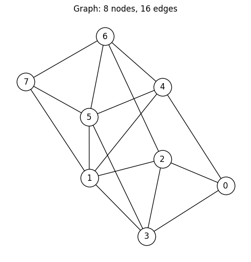

インスタンスの作成¶

グラフからエッジリストを取得し、JijModeling の問題を具体的なデータで評価します。

instance_data = {"V": num_nodes, "E": edge_list}
instance = problem.eval(instance_data)

QAOAConverter のセットアップ¶

QAOAConverter は OMMX インスタンスを受け取り、内部で以下を行います：

問題を QUBO（Quadratic Unconstrained Binary Optimization）形式に変換。
BINARY 変数から SPIN 変数へ変換。
Pauli-Z 演算子の和としてコストハミルトニアンを構築。

元の問題には制約があるため、QUBO 定式化では制約がペナルティ項として目的関数に組み込まれます。そのため、デコードされたサンプルのエネルギー値は元の目的関数（カットエッジ数）とは異なり、ペナルティを含んでいます。実行可能性の確認と真の目的関数値の計算を別途行う必要があります。

from qamomile.optimization.qaoa import QAOAConverter

converter = QAOAConverter(instance)
converter.spin_model = converter.spin_model.normalize_by_abs_max()
hamiltonian = converter.get_cost_hamiltonian()
print(hamiltonian)

Hamiltonian((Z0, Z1): 1.0, (Z0, Z5): 1.0, (Z0, Z6): 1.0, (Z0, Z7): 1.0, (Z1, Z6): 1.0, (Z2, Z4): 1.0, (Z2, Z5): 1.0, (Z2, Z7): 1.0, (Z3, Z4): 1.0, (Z3, Z6): 1.0, (Z3, Z7): 1.0, (Z4, Z7): 1.0)

実行可能な回路へのトランスパイル¶

converter.transpile() は p 層の QAOA アンザッツ回路を構築し、ExecutableProgram にコンパイルします。変分パラメータ gammas（コスト層）と betas（ミキサー層）はランタイムパラメータとして残ります。

from qamomile.qiskit import QiskitTranspiler

transpiler = QiskitTranspiler()
p = 5  # QAOA の層数
executable = converter.transpile(transpiler, p=p)

QAOA 回路の可視化¶

QAOAConverter._transpile_quadratic() は内部で次のサンプリング qkernel を組み立てて transpile します。チュートリアルでは可視化のため、その qkernel をそのままここに再掲します。Transpiler.to_block で IR ブロックに落とし、Transpiler.inline でサブ qkernel を展開してから MatplotlibDrawer.draw に渡すことで、コンバーターが内部で扱うのと同じ Block 構造を描画できます(レイヤー構造を読みやすくするため p=2 に縮小)。

import qamomile.circuit as qmc
from qamomile.circuit.algorithm.qaoa import qaoa_state
from qamomile.circuit.visualization import MatplotlibDrawer


@qmc.qkernel
def qaoa_sampling(
    p: qmc.UInt,
    quad: qmc.Dict[qmc.Tuple[qmc.UInt, qmc.UInt], qmc.Float],
    linear: qmc.Dict[qmc.UInt, qmc.Float],
    gammas: qmc.Vector[qmc.Float],
    betas: qmc.Vector[qmc.Float],
    n: qmc.UInt,
) -> qmc.Vector[qmc.Bit]:
    q = qaoa_state(p=p, quad=quad, linear=linear, n=n, gammas=gammas, betas=betas)
    return qmc.measure(q)


block = transpiler.to_block(
    qaoa_sampling,
    bindings={
        "linear": converter.spin_model.linear,
        "quad": converter.spin_model.quad,
        "n": converter.spin_model.num_bits,
        "p": 2,
    },
    parameters=["gammas", "betas"],
)
block = transpiler.inline(block)
# `fold_loops=False` で全ループ(`for layer`/`for (i,j),Jij in quad`/`for i in range(n)`)を
# アンロールして、各ゲートを展開した形で描画する。`linear` は空辞書 `{}` のため、
# `for i, hi in linear` は 0 イテレーションとして消える(ボックスは現れない)。
# 結果は横長になるが、ドキュメントビルド時にライトボックス用 JS が注入されるので、
# クリックでモーダル拡大表示できる。
MatplotlibDrawer(block).draw(fold_loops=False)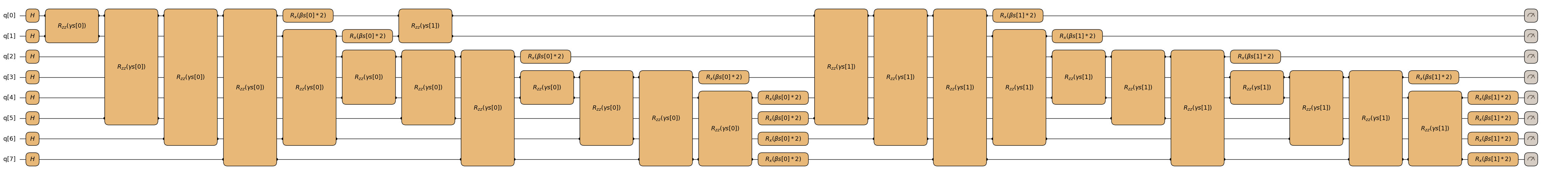

内部の構成要素を見る¶

qaoa_sampling の中では qaoa_state を呼んでいますが、qaoa_state 自体は次の3つの組み合わせで構成されています:

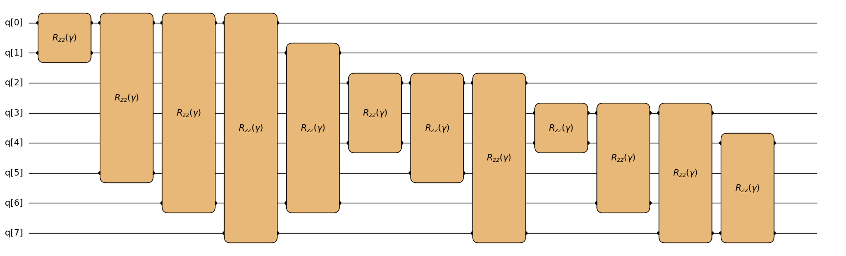
superposition_vector(n) — 全ビットに H を作用させて初期状態 $|+\rangle^{\otimes n}$ を準備する。
ising_cost(quad, linear, q, gamma) — 二次項 quad の各エントリに対して RZZ、線形項 linear の各エントリに対して RZ を作用させるコスト層。今回の問題では線形項がない(linear={})ので RZZ だけが現れる。
x_mixer(q, beta) — 全ビットに RX(2\beta) を作用させるミキサー層。

qaoa_layers(p, ...) はこの ising_cost と x_mixer を p 回交互に作用させているだけです。各部品を個別に描画して中身を確認します。

from qamomile.circuit.algorithm.basic import superposition_vector
from qamomile.circuit.algorithm.qaoa import ising_cost, x_mixer

superposition_vector.draw(n=converter.spin_model.num_bits, fold_loops=False)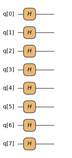

ising_cost.draw(
    q=converter.spin_model.num_bits,
    quad=converter.spin_model.quad,
    linear=converter.spin_model.linear,
    fold_loops=False,
)

x_mixer.draw(q=converter.spin_model.num_bits, fold_loops=False)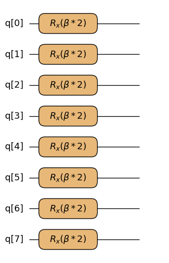

QAOA パラメータの最適化¶

executable.sample() を使って各イテレーションでコストを評価します。オプティマイザはサンプリングされたビット列の平均エネルギーを最小化する gammas と betas を探索します。

import os
import numpy as np
from qiskit_aer import AerSimulator
from scipy.optimize import minimize

# シミュレータをseedしておくことで、notebookを再実行してもCOBYLAの軌道と
# 最終的なサンプリング分布が再現される。seedなしの場合、ショットごとに
# 異なる乱数が引かれるためCOBYLAはノイズのあるコスト面を辿り、
# 実行のたびに(等価ではあるが)異なる局所最適解に収束する。
executor = transpiler.executor(
    backend=AerSimulator(seed_simulator=901, max_parallel_threads=1)
)
docs_test_mode = os.environ.get("QAMOMILE_DOCS_TEST") == "1"
sample_shots = 256 if docs_test_mode else 2048
maxiter = 25 if docs_test_mode else 1000

rng = np.random.default_rng(900)
initial_params = rng.uniform(0, np.pi, 2 * p)

cost_history = []


def cost_fn(params):
    gammas = list(params[:p])
    betas = list(params[p:])
    job = executable.sample(
        executor,
        shots=sample_shots,
        bindings={"gammas": gammas, "betas": betas},
    )
    result = job.result()
    # decode_to_binary_sampleset は QUBO ドメインの BinarySampleSet を返す。
    # その `energy` はペナルティを含む目的関数値で、COBYLA が実行不可能解の
    # コストを認識するために必要。多態的な decode() が返す ommx.v1.SampleSet
    # の `objective` はペナルティを含まない真の目的関数値であり、
    # 最適化器を実行不可能な全 0/全 1 ビット列に収束させてしまう。
    decoded = converter.decode_to_binary_sampleset(result)
    energy = decoded.energy_mean()
    cost_history.append(energy)
    return energy


res = minimize(
    cost_fn,
    initial_params,
    method="COBYLA",
    options={"maxiter": maxiter},
)

print(f"Optimized cost: {res.fun:.3f}")
print(f"Optimal params: {[round(v, 4) for v in res.x]}")
print(f"Function evaluations: {res.nfev}")

Optimized cost: 14.235
Optimal params: [np.float64(0.5042), np.float64(0.9744), np.float64(3.1558), np.float64(0.7789), np.float64(2.1748), np.float64(1.1239), np.float64(3.6516), np.float64(1.5606), np.float64(1.5563), np.float64(0.7607)]
Function evaluations: 117

plt.figure(figsize=(8, 4))
plt.plot(cost_history, color="#2696EB")
plt.xlabel("Iteration")
plt.ylabel("Cost (mean energy)")
plt.title("QAOA Optimization Progress")
plt.show()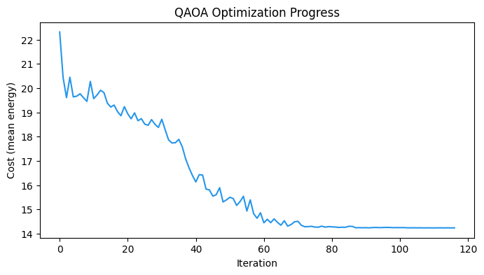

最適化されたパラメータでサンプリング¶

最適化されたパラメータを使い、回路をサンプリングしてビット列として候補解を取得します。

gammas_opt = list(res.x[:p])
betas_opt = list(res.x[p:])

sample_result = executable.sample(
    executor,
    shots=1000,
    bindings={"gammas": gammas_opt, "betas": betas_opt},
).result()

# OMMXベースのコンバーターで`decode()`を呼ぶと、元の(ペナルティを含まない)
# インスタンスで評価された`ommx.v1.SampleSet`が返る。実行可能性、真の目的関数値、
# 制約ごとの違反量がOMMXのAPIから直接得られるため、自前の実行可能性判定や
# 目的関数値計算ヘルパーは不要。
sample_set = converter.decode(sample_result)

結果の分析¶

実行可能性のチェック¶

QAOAのサンプルは候補解であり、元の制約を満たすとは限りません。制約 $\sum x_u = |V|/2$ はQUBOのペナルティとして組み込まれているため、制約を満たさないビット列も出力に含まれる可能性があります。

SampleSet.summaryはショットごとに1行を持つDataFrameで、feasible列には元の制約に対する実行可能性がすでに格納されています。実行可能なショット数はそこから直接取得できます。

summary = sample_set.summary
total_feasible = int(summary["feasible"].sum())
total_samples = len(summary)

print(
    f"Feasible samples: {total_feasible} / {total_samples} "
    f"({100 * total_feasible / total_samples:.1f}%)"
)

Feasible samples: 538 / 1000 (53.8%)

最良の実行可能解¶

SampleSet.best_feasibleは、実行可能解のうち目的関数値が最良(ここでは最小)のものを返します。コンバーターをOMMXのInstanceから構築しているため、報告される目的関数値は元のペナルティを含まないもの、すなわちカットエッジ数そのものです。決定変数の値はdecision_variables_dfに元の変数IDをキーとして格納されています。

if total_feasible > 0:
    best = sample_set.best_feasible
    best_obj = int(round(best.objective))
    best_sample = {
        i: int(round(best.decision_variables_df.loc[i, "value"]))
        for i in range(num_nodes)
    }
    print(f"Best feasible solution: {best_sample}")
    print(f"Cut edges:             {best_obj}")
else:
    print("No feasible solution found. Try increasing p or maxiter.")
    best_sample = None
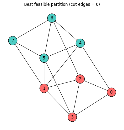
    best_obj = None

Best feasible solution: {0: 1, 1: 1, 2: 1, 3: 1, 4: 0, 5: 0, 6: 0, 7: 0}
Cut edges:             6

目的関数値の分布¶

実行可能なサンプルのみについて、真の目的関数値(カットエッジ数)の分布を表示します。summaryにはショットごとに元の目的関数値が格納されているため、実行可能なスライスに対してvalue_counts()を呼ぶだけで分布が得られます。

if total_feasible > 0:
    feasible_objectives = (
        summary.loc[summary["feasible"], "objective"].round().astype(int)
    )
    obj_counts = feasible_objectives.value_counts().sort_index()

    plt.figure(figsize=(8, 4))
    plt.bar([str(o) for o in obj_counts.index], obj_counts.values, color="#2696EB")
    plt.xlabel("Cut edges (objective value)")
    plt.ylabel("Frequency")
    plt.title("Distribution of Feasible Solutions")
    plt.show()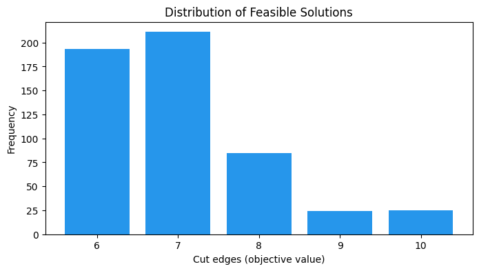

最良の分割の可視化¶

QAOA が見つけた最良の実行可能な分割に基づいて、グラフのノードを色分けします。

if best_sample is not None:
    color_map = [
        "#FF6B6B" if best_sample.get(i, 0) == 1 else "#4ECDC4" for i in range(num_nodes)
    ]

    plt.figure(figsize=(5, 5))
    nx.draw(
        G,
        pos,
        with_labels=True,
        node_color=color_map,
        node_size=700,
        edgecolors="black",
    )
    plt.title(f"Best feasible partition (cut edges = {best_obj})")
    plt.show()