実行モデル：sample()とrun()

タグ: tutorial

Qamomileは量子カーネルの戻り値に応じて2つの実行メソッドを提供します：

量子カーネルの戻り値	使用メソッド	返される結果
`Bit`, `Vector[Bit]`, `tuple[Bit, ...]`	`sample()`	`SampleResult` — カウント付き測定結果
`Float` (`expval`から)	`run()`	`float` — 期待値

この章では両方のメソッドを説明し、期待値計算のためのオブザーバブルを紹介します。

# 最新のQamomileをpipからインストールします！
# !pip install qamomile

import math

import qamomile.circuit as qmc
import qamomile.observable as qmo
from qamomile.qiskit import QiskitTranspiler

transpiler = QiskitTranspiler()

複数量子ビットの`sample()`¶

チュートリアル01では単一のBitをサンプリングしました。量子カーネルが複数ビットを返す場合、各測定結果は整数値（0または1）のタプルになります。

@qmc.qkernel
def parity_probe(theta: qmc.Float) -> tuple[qmc.Bit, qmc.Bit]:
    q0 = qmc.qubit(name="q0")
    q1 = qmc.qubit(name="q1")

    q0 = qmc.h(q0)
    q1 = qmc.ry(q1, theta)
    q0, q1 = qmc.cx(q0, q1)

    return qmc.measure(q0), qmc.measure(q1)

parity_probe.draw(theta=0.7)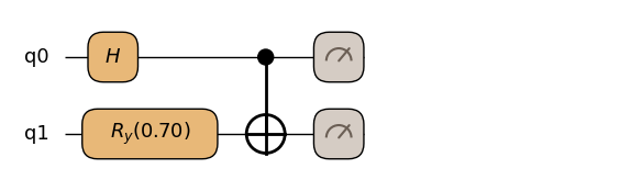

exe_sample = transpiler.transpile(parity_probe, parameters=["theta"])
sample_result = exe_sample.sample(
    transpiler.executor(),
    shots=256,
    bindings={"theta": 0.7},
).result()

for outcome, count in sample_result.results:
    print(f"  outcome={outcome}, count={count}")
assert sample_result.shots == 256
assert sum(count for _, count in sample_result.results) == 256
# parity_probe は tuple[Bit, Bit] を返す → 各 outcome は 2 要素 tuple。
assert all(
    isinstance(outcome, tuple) and len(outcome) == 2
    for outcome, _ in sample_result.results
)

  outcome=(1, 0), count=19
  outcome=(0, 1), count=23
  outcome=(0, 0), count=108
  outcome=(1, 1), count=106

各outcomeは(0, 1)や(1, 0)のようなタプルです。最初の要素はq0に、2番目の要素はq1に対応し、return文での順序と一致します。

ビット順序の規約¶

Qamomileの出力はビッグエンディアン順序を使用します：最も左の位置が戻り値タプルの最初の量子ビットに対応します。

(measure(q0), measure(q1), measure(q2))を返す量子カーネルの場合：

結果タプル	q0	q1	q2
`(0, 1, 1)`	0	1	1
`(1, 0, 0)`	1	0	0

タプルの位置iが戻り値の量子ビットiに対応します。

注意：Qiskitは内部的にリトルエンディアンを使用しますが、Qamomileが変換を処理します。結果は常に記述した順序で得られます。

期待値が必要な場合¶

個々の測定結果ではなく、量子オブザーバブルの期待値（平均値）が必要な場面があります。例えば：

VQE（変分量子固有値ソルバー）： $\langle \psi \rvert H \lvert \psi \rangle$ の最小化
QAOA：コスト関数の期待値の評価
量子パラメータに対するあらゆる最適化ループ

このためにQamomileはexpval()とrun()を提供しています。

Observable型¶

関連する2つの概念があります：

qmc.Observable — 量子カーネルのシグネチャで使用するハンドル型です。qmc.Floatと同様に、量子カーネルの引数や戻り値の型アノテーションで使用します。
qamomile.observableモジュール — バインディングで渡す具体的なオブザーバブル値を構築する場所です。例えば

import qamomile.observable as qmo

H = qmo.Z(0)                        # 量子ビット0のパウリZ
H = qmo.Z(0) * qmo.Z(1)             # ZZ相互作用
H = 0.5 * qmo.X(0) + 0.3 * qmo.Y(1) # 線形結合

`expval()`:オブザーバブルの測定¶

expval(qubit, hamiltonian)は期待値 $\langle \psi \rvert H \lvert \psi \rangle$ （ $\lvert \psi \rangle$ はqubitを表し、 $H$ はhamiltonianに対応）を計算し、qmc.Floatを返します。expvalからFloatを返す量子カーネルはrun()で実行する必要があります。

@qmc.qkernel
def z_expectation(theta: qmc.Float, hamiltonian: qmc.Observable) -> qmc.Float:
    q = qmc.qubit(name="q")
    q = qmc.ry(q, theta)
    return qmc.expval(q, hamiltonian)


H = qmo.Z(0)

z_expectation.draw(theta=0.7, hamiltonian=H)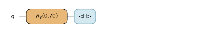

`run()`による実行¶

期待値を返す量子カーネルにはsample()の代わりにrun()を使います。オブザーバブルはトランスパイル時にバインドし（測定回路に影響するため）、thetaはスイープ可能なパラメータとして残します。

exe_run = transpiler.transpile(
    z_expectation,
    bindings={"hamiltonian": H},  # Observable bound at transpile time
    parameters=["theta"],  # theta remains sweepable
)

run_result = exe_run.run(
    transpiler.executor(),
    bindings={"theta": 0.7},
).result()

print("expectation value:", run_result)
print("python type:", type(run_result))
assert isinstance(run_result, float)
# Ry(theta)|0> の <Z> は厳密に cos(theta)。statevector estimator は
# 浮動小数点精度で返す。
assert math.isclose(run_result, math.cos(0.7), abs_tol=1e-10)

expectation value: 0.7648421872844884
python type: <class 'float'>

run().result()はプレーンなfloatを返します — 推定された $\langle \psi \rvert Z \lvert \psi \rangle$ の値です。 $\theta = 0.7$ の場合、RYゲートが量子ビットを

R_Y(\theta) \lvert 0 \rangle = \cos\left( \frac{\theta}{2} \right) \lvert 0 \rangle + \sin\left( \frac{\theta}{2} \right) \lvert 1 \rangle

(1)

のように回転させ、Zの期待値は $\cos^2\left( \frac{\theta}{2} \right) - \sin^2\left( \frac{\theta}{2} \right) = \cos(\theta) \approx 0.765$ となります。

`sample()`と`run()`¶

量子カーネルの戻り値	実行メソッド	`.result()`の返り値
`Bit`	`sample()`	`SampleResult` (`.results: list[tuple[int, int]]`)
`tuple[Bit, Bit]`	`sample()`	`SampleResult` (`.results: list[tuple[tuple[int, int], int]]`)
`Vector[Bit]`	`sample()`	`SampleResult` (`.results: list[tuple[tuple[int, ...], int]]`)
`Float` (`expval`から)	`run()`	`float`

使い分け：量子カーネルがmeasure()で終わる場合はsample()を使用します。expval()で終わる場合はrun()を使用します。

まとめ¶

sample()は測定ビットを返す量子カーネル用 — カウント付きの測定結果分布が得られます。
run()はexpval()でFloatを返す量子カーネル用 — 単一の期待値が得られます。
qmc.Observableはハンドル型、qamomile.observable.Z(0)等が具体的な値です。オブザーバブルはトランスパイル時にバインドします。
ビット順序はビッグエンディアン：戻り値タプルの位置が量子ビットの順序に対応します。

次へ：古典フローパターン — qmc.rangeによるループ、qmc.itemsによるスパースデータ、条件分岐。

複数量子ビットのsample()¶