タグ: tutorial resource-estimation
このチュートリアルでは、量子カーネルを実行せずに論理リソースを推定し、その結果を読み取る方法を学びます。具体的には、次の内容を扱います。
パラメータなし・パラメータ付きの量子カーネルを推定する
量子ビット幅、ゲート数・測定・リセット数、深さを確認する
本体を持たないOracleへ固定costまたはcallbackを設定する
controlの分解方法と、costが不明なOracleの扱いを選ぶ
derivation、quality、approximation、assumptionsから推定結果の意味を確認する
最後のAppendixには、ResourceEstimateで確認できる全フィールドをまとめます。
# 最新のQamomileをpipからインストールします!
# !pip install "qamomile[visualization]"
このチュートリアルで使うライブラリをimportします。
import sympy as sp

import qamomile.circuit as qmc
import qamomile.observable as qmo
1. リソース推定を実行する
estimate_resources()を使うと、量子カーネルを実行したり、特定のengine向けにtranspileしたりせずに、量子アルゴリズム上の論理リソースを見積もれます。パラメータ付きの量子カーネルも、パラメータを固定せずに推定できます。
1.1 パラメータなしの量子カーネルを推定する
最初に、Bell状態を準備して2個の量子ビットを測定する量子カーネルを定義します。
@qmc.qkernel
def bell_pair() -> tuple[qmc.Bit, qmc.Bit]:
    """Prepare and measure one Bell pair."""
    control = qmc.qubit("control")
    target = qmc.qubit("target")

    control = qmc.h(control)
    control, target = qmc.cx(control, target)

    return qmc.measure(control), qmc.measure(target)


bell_pair.draw()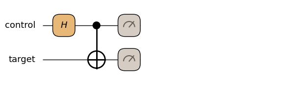
量子カーネルのestimate_resources()を呼び出すと、ResourceEstimateが返ります。これは量子カーネルを実行して得る測定結果ではありません。Qamomileが量子カーネルから、量子ビット幅、論理ゲート・測定・リセット数、深さなどを数えた結果です。ここでは代表的な値だけを表示します。
bell_estimate = bell_pair.estimate_resources()

print("量子ビット数:", bell_estimate.qubits)
print("総ゲート数:", bell_estimate.gates.total)
print("1量子ビットゲート数:", bell_estimate.gates.single_qubit)
print("2量子ビットゲート数:", bell_estimate.gates.two_qubit)
print("測定数:", bell_estimate.measurements.total)
print("深さ:", bell_estimate.depth.depth)
print("ゲートの深さ:", bell_estimate.depth.gate_depth)

assert bell_estimate.qubits - 2 == 0
assert bell_estimate.gates.total - 2 == 0
assert bell_estimate.gates.single_qubit - 1 == 0
assert bell_estimate.gates.two_qubit - 1 == 0
assert bell_estimate.measurements.total - 2 == 0
assert bell_estimate.depth.depth - 3 == 0
assert bell_estimate.depth.gate_depth - 2 == 0
量子ビット数: 2
総ゲート数: 2
1量子ビットゲート数: 1
2量子ビットゲート数: 1
測定数: 2
深さ: 3
ゲートの深さ: 2
bell_pairでは、2個の量子ビット、HadamardゲートとCXゲートの合計2個のゲート、2回の測定が必要です。ゲート列の後に測定レイヤーがあるため、全体の深さは3です。
1.2 パラメータ付き量子カーネルを推定する
Bell状態は、2個の量子ビットからなるGHZ(Greenberger–Horne–Zeilinger)状態と考えられます。これをn個の量子ビットからなるGHZ状態へ一般化しましょう。最初の量子ビットへHadamardゲートを適用し、隣り合う量子ビットをCXゲートで順番に接続します。
@qmc.qkernel
def ghz_state(n: qmc.UInt) -> qmc.Vector[qmc.Bit]:
    """Prepare and measure a GHZ state with a symbolic width."""
    qubits = qmc.qubit_array(n, "qubits")
    qubits[0] = qmc.h(qubits[0])
    for index in qmc.range(n - 1):
        qubits[index], qubits[index + 1] = qmc.cx(
            qubits[index],
            qubits[index + 1],
        )
    return qmc.measure(qubits)


ghz_state.draw(n=4, fold_loops=False)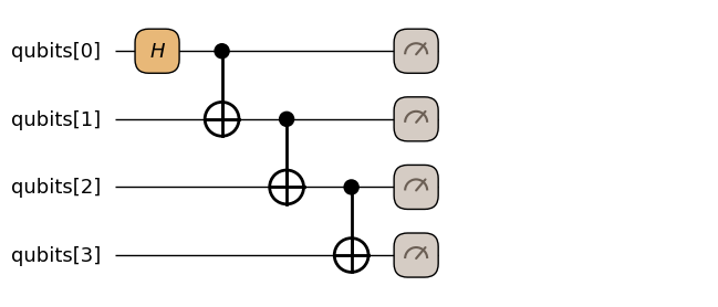
nの値を渡さなくても、シンボリックにリソースを推定できます。
ghz_symbolic_estimate = ghz_state.estimate_resources()

print("パラメータ:", ghz_symbolic_estimate.parameters)
print("量子ビット数:", ghz_symbolic_estimate.qubits)
print("総ゲート数:", ghz_symbolic_estimate.gates.total)
print("1量子ビットゲート数:", ghz_symbolic_estimate.gates.single_qubit)
print("2量子ビットゲート数:", ghz_symbolic_estimate.gates.two_qubit)
print("測定数:", ghz_symbolic_estimate.measurements.total)
print("深さ:", ghz_symbolic_estimate.depth.depth)
print("ゲートの深さ:", ghz_symbolic_estimate.depth.gate_depth)

n = ghz_symbolic_estimate.parameters["n"]
cx_count = n - 1
expected_depth = n + 1

assert sp.simplify(ghz_symbolic_estimate.qubits - n) == 0
assert sp.simplify(ghz_symbolic_estimate.gates.total - (cx_count + 1)) == 0
assert sp.simplify(ghz_symbolic_estimate.gates.single_qubit - 1) == 0
assert sp.simplify(ghz_symbolic_estimate.gates.two_qubit - cx_count) == 0
assert sp.simplify(ghz_symbolic_estimate.measurements.total - n) == 0
assert sp.simplify(ghz_symbolic_estimate.depth.depth - expected_depth) == 0
assert sp.simplify(ghz_symbolic_estimate.depth.gate_depth - (cx_count + 1)) == 0
assert ghz_symbolic_estimate.quality is qmc.EstimateQuality.CONSERVATIVE
assert any(
    assumption.source == "qkernel input domain"
    and "n >= 1" in assumption.message
    for assumption in ghz_symbolic_estimate.assumptions
)
パラメータ: {'n': n}
量子ビット数: n
総ゲート数: n
1量子ビットゲート数: 1
2量子ビットゲート数: n - 1
測定数: n
深さ: n + 1
ゲートの深さ: n
1.3 特定の入力で具体化する
特定の入力に対する具体的な値が必要な場合は、推定時にinputsを渡す方法と、すでに得たシンボリックな推定結果へ.substitute()を適用する方法があります。
| 方法 | 値を使うタイミング | 適した用途 |
|---|---|---|
estimate_resources(inputs={...}) | リソース推定を行うとき | 配列shape、index、branch、loop構造などを最初から具体化したい場合 |
estimate.substitute(...) | すでに得た推定式を評価するとき | 同じシンボリックな推定結果を複数の問題サイズで比較したい場合 |
まず、inputsを使って、推定を始める時点でn=4を具体化します。
ghz_input_estimate = ghz_state.estimate_resources(
    inputs={"n": 4},
)

print("inputs → 量子ビット数:", ghz_input_estimate.qubits)
print("inputs → 総ゲート数:", ghz_input_estimate.gates.total)

assert ghz_input_estimate.qubits - 4 == 0
assert ghz_input_estimate.gates.total - 4 == 0
assert ghz_input_estimate.gates.single_qubit - 1 == 0
assert ghz_input_estimate.gates.two_qubit - (4 - 1) == 0
assert ghz_input_estimate.measurements.total - 4 == 0
assert ghz_input_estimate.depth.depth - (4 + 1) == 0
assert ghz_input_estimate.depth.gate_depth - 4 == 0
inputs → 量子ビット数: 4
inputs → 総ゲート数: 4
次に、すでに得たghz_symbolic_estimateへ.substitute(n=4)を適用します。この方法では、量子カーネルを再解析せず、完成している推定式のnを4へ置き換えます。
ghz_substituted_estimate = ghz_symbolic_estimate.substitute(n=4)

print("substitute → 量子ビット数:", ghz_substituted_estimate.qubits)
print("substitute → 総ゲート数:", ghz_substituted_estimate.gates.total)

assert ghz_substituted_estimate.qubits - ghz_input_estimate.qubits == 0
assert ghz_substituted_estimate.gates.total - ghz_input_estimate.gates.total == 0
assert (
    ghz_substituted_estimate.gates.single_qubit - ghz_input_estimate.gates.single_qubit
    == 0
)
assert (
    ghz_substituted_estimate.gates.two_qubit - ghz_input_estimate.gates.two_qubit == 0
)
assert (
    ghz_substituted_estimate.measurements.total - ghz_input_estimate.measurements.total
    == 0
)
assert ghz_substituted_estimate.depth.depth - ghz_input_estimate.depth.depth == 0
assert (
    ghz_substituted_estimate.depth.gate_depth - ghz_input_estimate.depth.gate_depth == 0
)
substitute → 量子ビット数: 4
substitute → 総ゲート数: 4
ghz_stateでは、どちらの方法でも量子ビット数、ゲート数、測定数、深さは同じです。ただし、値を適用するタイミングが異なるため、どの量子カーネルでも同じ結果になるとは限りません。
.substitute()は、すでに得た推定式を置換するだけで、量子ビット間の依存関係や深さを再計算しません。二つの方法で違いが現れる例として、qubits[0]へHadamardゲートを適用した後、シンボリックなindexを使ってqubits[i]へXゲートを適用する場合を考えます。
@qmc.qkernel
def symbolic_access(i: qmc.UInt) -> qmc.Vector[qmc.Qubit]:
    """Access qubits[0] and qubits[i] in a symbolic way."""
    qubits = qmc.qubit_array(i + 1, "qubits")
    qubits[0] = qmc.h(qubits[0])
    qubits[i] = qmc.x(qubits[i])
    return qubits


symbolic_access.draw(i=1)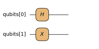
iを指定せずに推定すると、二つのゲートが同じ量子ビットへ作用する可能性があるため、安全側に直列化して深さ2と推定します。
access_symbolic_estimate = symbolic_access.estimate_resources()

print("シンボリック → 深さ:", access_symbolic_estimate.depth.depth)
assert access_symbolic_estimate.depth.depth - 2 == 0
シンボリック → 深さ: 2
inputs={"i": 0}を推定時に渡すと、二つのゲートが同じ量子ビットへ作用すると分かるため、深さは2です。
access_i0_estimate = symbolic_access.estimate_resources(inputs={"i": 0})

print("inputs、i=0 → 深さ:", access_i0_estimate.depth.depth)
assert access_i0_estimate.depth.depth - 2 == 0
inputs、i=0 → 深さ: 2
inputs={"i": 1}を推定時に渡すと、二つのゲートが異なる量子ビットへ作用すると分かり、並列に配置できるため深さは1です。
access_i1_estimate = symbolic_access.estimate_resources(inputs={"i": 1})

print("inputs、i=1 → 深さ:", access_i1_estimate.depth.depth)
assert access_i1_estimate.depth.depth - 1 == 0
inputs、i=1 → 深さ: 1
一方、シンボリックな推定結果へ.substitute(i=1)を適用しても、すでに決まった順序関係は再計算されません。そのため、式の値を置き換えた後も深さは2のままです。
access_i1_substituted_estimate = access_symbolic_estimate.substitute(i=1)

print("substitute、i=1 → 深さ:", access_i1_substituted_estimate.depth.depth)
assert access_i1_substituted_estimate.depth.depth - 2 == 0
substitute、i=1 → 深さ: 2
2. よく使う推定結果を読む
estimate_resources()が返すResourceEstimateでは、量子ビット幅(.width)、量子ゲート数・測定・リセット数(.gates/.measurements/.resets)、深さ(.depth)が項目別に格納されています。ここでは、普段よく確認する項目に絞って紹介します。全フィールドはAppendixにまとめます。
2.1 量子ビット幅
量子ビット幅には、次の項目があります。
width.input_qubits:呼び出し側から量子カーネルへ渡される量子ビット数width.allocated_qubits:量子カーネルの本体で確保する量子ビット数width.clean_ancilla_qubits:初期状態が|0>である必要がある補助量子ビット数width.peak_qubits:実行中に同時に必要になる論理量子ビットの最大数width.circuit_qubits:入力、すべての確保場所、clean/dirty ancillaを合わせた静的な回路幅
ResourceEstimate.qubitsはwidth.peak_qubitsのalias、ResourceEstimate.circuit_qubitsはwidth.circuit_qubitsのaliasです。第1章の4個の量子ビットからなるghz_stateを使って、これらの値を確認します。
ghz_estimate = ghz_state.estimate_resources(inputs={"n": 4})

print("ピーク量子ビット数:", ghz_estimate.qubits)
print("入力量子ビット数:", ghz_estimate.width.input_qubits)
print("確保する量子ビット数:", ghz_estimate.width.allocated_qubits)
print("clean ancilla数:", ghz_estimate.width.clean_ancilla_qubits)
print("静的な回路幅:", ghz_estimate.circuit_qubits)

assert ghz_estimate.qubits - 4 == 0
assert ghz_estimate.width.input_qubits - 0 == 0
assert ghz_estimate.width.allocated_qubits - 4 == 0
assert ghz_estimate.width.clean_ancilla_qubits - 0 == 0
assert ghz_estimate.circuit_qubits - 4 == 0
ピーク量子ビット数: 4
入力量子ビット数: 0
確保する量子ビット数: 4
clean ancilla数: 0
静的な回路幅: 4
ghz_stateは量子ビットを引数として受け取らず、本体で4個確保します。この例では4個すべてを同時に使い、追加のancillaも必要ないため、ピーク幅と静的な回路幅はどちらも4です。
qubitsとcircuit_qubitsは異なる場合があります。次の量子カーネルでは、最初の量子ビットを測定してその生存期間を終えた後に、別の量子ビットを確保します。
@qmc.qkernel
def released_qubit_example() -> qmc.Qubit:
    """Measure one qubit before allocating its replacement."""
    first = qmc.qubit("first")
    _measured = qmc.measure(first)
    return qmc.qubit("second")
released_qubit_estimate = released_qubit_example.estimate_resources()
print("ピーク量子ビット数:", released_qubit_estimate.qubits)
print("確保する量子ビット数:", released_qubit_estimate.width.allocated_qubits)
print("静的な回路幅:", released_qubit_estimate.circuit_qubits)
assert released_qubit_estimate.qubits - 1 == 0
assert released_qubit_estimate.width.allocated_qubits - 2 == 0
assert released_qubit_estimate.circuit_qubits - 2 == 0ピーク量子ビット数: 1
確保する量子ビット数: 2
静的な回路幅: 2
二つの量子ビットを同時には使わないため、ピーク幅は1です。一方、静的な回路では二つの確保場所を保持するため、circuit_qubitsは2です。
2.2 ゲート・測定・リセット数
ゲート数のフィールドでは、総数に加えて、作用する量子ビット数ごとの内訳を確認できます。例えば、multi_qubitは、3個以上の量子ビットへ作用する論理ゲートを数えます。
本体を解析できる通常の量子カーネルでは、作用する量子ビット数ごとの内訳を足すとtotalと一致します。
print("総ゲート数:", ghz_estimate.gates.total)
print("1量子ビットゲート数:", ghz_estimate.gates.single_qubit)
print("2量子ビットゲート数:", ghz_estimate.gates.two_qubit)
print("多量子ビットゲート数:", ghz_estimate.gates.multi_qubit)

assert ghz_estimate.gates.total - 4 == 0
assert ghz_estimate.gates.single_qubit - 1 == 0
assert ghz_estimate.gates.two_qubit - 3 == 0
assert ghz_estimate.gates.multi_qubit - 0 == 0
assert (
    ghz_estimate.gates.total
    - (
        ghz_estimate.gates.single_qubit
        + ghz_estimate.gates.two_qubit
        + ghz_estimate.gates.multi_qubit
    )
    == 0
)
総ゲート数: 4
1量子ビットゲート数: 1
2量子ビットゲート数: 3
多量子ビットゲート数: 0
4個の量子ビットからなるghz_stateには、1個のHadamardゲートと3個のCXゲートがあります。そのため、single_qubitは1、two_qubitは3、総ゲート数のtotalは4です。
測定とリセットはゲートに含めず、独立したフィールドとして数えます。
print("測定数:", ghz_estimate.measurements.total)
print("リセット数:", ghz_estimate.resets.total)

assert ghz_estimate.measurements.total - 4 == 0
assert ghz_estimate.resets.total - 0 == 0
測定数: 4
リセット数: 0
4個の量子ビットを測定するため、measurements.totalは4です。この量子カーネルにはリセットを書いていないため、resets.totalは0です。これは量子ビットごとの測定イベント数であり、shots数は掛けません。
2.3 深さ
ゲート数が論理ゲートの実行回数を表すのに対し、深さは依存関係を守りながら何層に配置できるかを表します。
depth.depthは量子カーネル全体のクリティカルパスの長さです。クリティカルパスとは、依存関係によって実行順序を変えられない演算の連鎖のうち、レイヤー数が最大になるものです。gate_depth、measurement_depth、reset_depthは、同じ依存関係を保ったまま、それぞれゲート、測定、リセットだけがレイヤー数に寄与する深さです。一般には、種類ごとの深さを足してdepth.depthを復元することはできません。
print("全体の深さ:", ghz_estimate.depth.depth)
print("ゲートの深さ:", ghz_estimate.depth.gate_depth)
print("測定の深さ:", ghz_estimate.depth.measurement_depth)
print("リセットの深さ:", ghz_estimate.depth.reset_depth)

assert ghz_estimate.depth.depth - 5 == 0
assert ghz_estimate.depth.gate_depth - 4 == 0
assert ghz_estimate.depth.measurement_depth - 1 == 0
assert ghz_estimate.depth.reset_depth - 0 == 0
全体の深さ: 5
ゲートの深さ: 4
測定の深さ: 1
リセットの深さ: 0
ghz_stateでは、同じ量子ビットの状態を順に伝えるため、Hadamardゲートと3個のCXゲートは4層になります。その後に測定レイヤーが1つ必要なので、全体の深さは5です。
一方、異なる量子ビットに作用して依存関係を持たないゲートは、同じレイヤーへ配置できます。次の量子カーネルではHadamardゲートを2個使いますが、並列に実行できるためゲートの深さは1です。
@qmc.qkernel
def parallel_hadamards() -> qmc.Vector[qmc.Bit]:
    """Apply two independent Hadamard gates and measure both qubits."""
    qubits = qmc.qubit_array(2, "qubits")
    qubits[0] = qmc.h(qubits[0])
    qubits[1] = qmc.h(qubits[1])
    return qmc.measure(qubits)


parallel_hadamards.draw()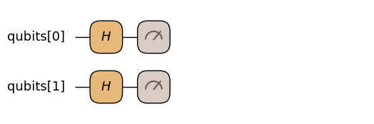
parallel_estimate = parallel_hadamards.estimate_resources()

print("総ゲート数:", parallel_estimate.gates.total)
print("ゲートの深さ:", parallel_estimate.depth.gate_depth)
print("測定数:", parallel_estimate.measurements.total)
print("測定の深さ:", parallel_estimate.depth.measurement_depth)
print("全体の深さ:", parallel_estimate.depth.depth)

assert parallel_estimate.gates.total - 2 == 0
assert parallel_estimate.depth.gate_depth - 1 == 0
assert parallel_estimate.measurements.total - 2 == 0
assert parallel_estimate.depth.measurement_depth - 1 == 0
assert parallel_estimate.depth.depth - 2 == 0
総ゲート数: 2
ゲートの深さ: 1
測定数: 2
測定の深さ: 1
全体の深さ: 2
2個のHadamardゲートは1つのゲートレイヤーに、2回の測定も1つの測定レイヤーに並べられます。そのため、ゲート数と測定数はそれぞれ2ですが、全体の深さは2です。
種類別の深さでも、対象外のゲートは順序関係から取り除かれません。次の量子カーネルでは、別々の量子ビットへ適用した二つのHadamardゲートを、間のRZZゲートが依存関係でつなぎます。
@qmc.qkernel
def category_depth_example() -> qmc.Vector[qmc.Qubit]:
    """Connect two Clifford gates through one rotation gate."""
    qubits = qmc.qubit_array(2, "qubits")
    qubits[0] = qmc.h(qubits[0])
    qubits[0], qubits[1] = qmc.rzz(qubits[0], qubits[1], 0.25)
    qubits[1] = qmc.h(qubits[1])
    return qubits


category_depth_example.draw()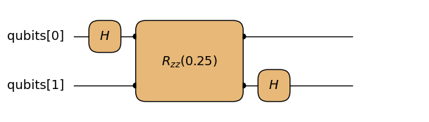
RZZゲートはclifford_depthのレイヤー数を増やしませんが、前後のHadamardゲートの依存関係をつなぎます。そのため、二つのHadamardゲートは別の量子ビットに作用していても、clifford_depthは2です。同様に、Hadamardゲートはrotation_depthやnon_clifford_depthのレイヤー数を増やしませんが、依存関係は保たれます。
category_depth_estimate = category_depth_example.estimate_resources()

print("全体の深さ:", category_depth_estimate.depth.depth)
print("ゲートの深さ:", category_depth_estimate.depth.gate_depth)
print("Cliffordの深さ:", category_depth_estimate.depth.clifford_depth)
print("回転ゲートの深さ:", category_depth_estimate.depth.rotation_depth)
print("non-Cliffordの深さ:", category_depth_estimate.depth.non_clifford_depth)

assert category_depth_estimate.depth.depth - 3 == 0
assert category_depth_estimate.depth.gate_depth - 3 == 0
assert category_depth_estimate.depth.clifford_depth - 2 == 0
assert category_depth_estimate.depth.rotation_depth - 1 == 0
assert category_depth_estimate.depth.non_clifford_depth - 1 == 0
全体の深さ: 3
ゲートの深さ: 3
Cliffordの深さ: 2
回転ゲートの深さ: 1
non-Cliffordの深さ: 1
3. Oracleにcostを設定する
通常の量子カーネルでは、Qamomileが本体の演算を再帰的にたどってリソースを推定します。一方、トップダウンで設計するときは、入出力だけを決めて、問題固有の処理をまだ実装しない場合があります。
このような処理は、実装を持たないqmc.Oracleとして表せます。推定に利用できる内部のゲート列がないため、既知のcostを固定値またはcallbackで設定します。
3.1 固定costを与える
1回の呼び出しに必要なcostが決まっている場合は、qmc.Oracleのcostへ固定のResourceEstimateを渡します。次のOracleは2個の量子ビットへ作用し、2個の1量子ビットゲートと3個の2量子ビットゲートを使うものとします。内部には一部のゲートを並列に実行できる箇所があり、ゲートの深さは4であることも分かっているとします。
固定costは、Oracleを通常どおり1回適用する場合のbase costです。costで省略したリソース項目は0として扱われます。ゲート数から内部の依存関係や並列性は復元できないため、深さも必要な場合はDepthResourcesとして明示します。
fixed_lookup = qmc.Oracle(
    "fixed_lookup",
    num_qubits=2,
    cost=qmc.ResourceEstimate(
        gates=qmc.GateResources(
            total=5,
            single_qubit=2,
            two_qubit=3,
        ),
        depth=qmc.DepthResources(
            depth=4,
            gate_depth=4,
        ),
    ),
)
Oracleは、量子カーネル内で通常の量子演算と同じように呼び出せます。
@qmc.qkernel
def with_fixed_oracle() -> qmc.Vector[qmc.Qubit]:
    """Apply one fixed-cost Oracle."""
    qs = qmc.qubit_array(2, "qs")
    return fixed_lookup(qs)


with_fixed_oracle.draw()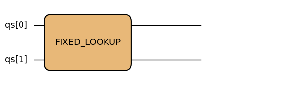
この量子カーネルを推定すると、Oracleへ設定した固定costに、呼び出し側で確保した2個の量子ビットが組み合わされます。
fixed_oracle_estimate = with_fixed_oracle.estimate_resources()

print("量子ビット数:", fixed_oracle_estimate.qubits)
print("総ゲート数:", fixed_oracle_estimate.gates.total)
print("1量子ビットゲート数:", fixed_oracle_estimate.gates.single_qubit)
print("2量子ビットゲート数:", fixed_oracle_estimate.gates.two_qubit)
print("ゲートの深さ:", fixed_oracle_estimate.depth.gate_depth)

assert fixed_oracle_estimate.qubits - 2 == 0
assert fixed_oracle_estimate.gates.total - 5 == 0
assert fixed_oracle_estimate.gates.single_qubit - 2 == 0
assert fixed_oracle_estimate.gates.two_qubit - 3 == 0
assert fixed_oracle_estimate.depth.depth - 4 == 0
assert fixed_oracle_estimate.depth.gate_depth - 4 == 0
量子ビット数: 2
総ゲート数: 5
1量子ビットゲート数: 2
2量子ビットゲート数: 3
ゲートの深さ: 4
推定結果には、Oracleへ指定した5個のゲートと深さ4がそのまま反映されています。2個の対象量子ビットは呼び出し側の量子カーネルが確保するため、ピーク幅は2です。
3.2 callbackでcostを計算する
受け取る量子ビット数が可変長の場合は、OracleのsignatureにCallableSignatureを指定します。また、受け取る量子ビット数などによってcostが変わる場合は、OpaqueCostContextを受け取るPython callbackを使ってcostを定義します。次のCallableSignatureは、可変長量子ビットvectorを1つ受け取り、vectorを1つ返す型を表します。このOracleのvector呼び出しでは、入力と同じshapeが出力にも引き継がれます。
callbackはリソース推定時に呼び出されます。context.target_qubitsから対象となる量子ビット数を参照でき、context.control_decompositionには現在のリソース推定で選択されたcontrol分解方法が入ります。
def parallel_hadamard_layer_cost(
    context: qmc.OpaqueCostContext,
) -> qmc.ResourceEstimate:
    """Return the cost of one parallel Hadamard layer."""
    target_qubits = context.target_qubits
    layer_depth = sp.Piecewise(
        (0, sp.Eq(target_qubits, 0)),
        (1, True),
    )
    return qmc.ResourceEstimate(
        gates=qmc.GateResources(
            total=target_qubits,
            single_qubit=target_qubits,
            clifford=target_qubits,
        ),
        depth=qmc.DepthResources(
            depth=layer_depth,
            gate_depth=layer_depth,
            clifford_depth=layer_depth,
        ),
        control_decomposition=context.control_decomposition,
    )


parallel_hadamard_layer = qmc.Oracle(
    "parallel_hadamard_layer",
    signature=qmc.CallableSignature(
        inputs=[qmc.Vector[qmc.Qubit]],
        outputs=[qmc.Vector[qmc.Qubit]],
    ),
    cost=parallel_hadamard_layer_cost,
)このcallbackは、対象となる各量子ビットへHadamardゲートを1個ずつ並列に適用するcostを返します。量子ビットが1個以上あれば、ゲート数は量子ビット数と同じですが、すべて同じレイヤーへ配置できるため深さは1です。返り値のcontrol_decompositionには、contextから受け取った設定を引き継いでいます。次に、このOracleを可変長量子ビット配列へ1回適用する量子カーネルを定義します。
@qmc.qkernel
def with_callback_oracle(width: qmc.UInt) -> qmc.Vector[qmc.Qubit]:
    """Apply an Oracle whose cost follows the array width."""
    qs = qmc.qubit_array(width, "qs")
    return parallel_hadamard_layer(qs)


with_callback_oracle.draw(width=4)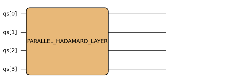
widthを指定せずに推定すると、callbackへシンボリックな対象幅が渡され、ゲート数と深さもシンボリックな式として返ります。
callback_oracle_estimate = with_callback_oracle.estimate_resources()

print("パラメータ:", callback_oracle_estimate.parameters)
print("総ゲート数:", callback_oracle_estimate.gates.total)
print("ゲートの深さ:", callback_oracle_estimate.depth.gate_depth)

width = callback_oracle_estimate.parameters["width"]
expected_layer_depth = sp.Piecewise(
    (0, sp.Eq(width, 0)),
    (1, True),
)
assert sp.simplify(callback_oracle_estimate.qubits - width) == 0
assert sp.simplify(callback_oracle_estimate.gates.total - width) == 0
assert sp.simplify(callback_oracle_estimate.gates.single_qubit - width) == 0
assert sp.simplify(callback_oracle_estimate.gates.clifford - width) == 0
assert sp.simplify(callback_oracle_estimate.depth.depth - expected_layer_depth) == 0
assert (
    sp.simplify(callback_oracle_estimate.depth.gate_depth - expected_layer_depth) == 0
)
assert (
    sp.simplify(callback_oracle_estimate.depth.clifford_depth - expected_layer_depth)
    == 0
)
パラメータ: {'width': width}
総ゲート数: width
ゲートの深さ: Piecewise((0, Eq(width, 0)), (1, True))
ゲート数にはシンボリックな対象幅が現れ、深さは対象が空なら0、それ以外なら1になります。
4. 推定方法を設定する
estimate_resources()には、推定対象の構造をどのようなmodelで数えるかを選ぶ設定があります。ここでは、controlの分解方法と、costが分からない処理の扱いを説明します。
4.1 control decomposition
control_decompositionは、制御演算をどのように数えるかを設定します。既定値のCLEAN_ANCILLA_TOFFOLIは、Toffoliゲートと初期状態が|0>のclean ancillaを使う固定の分解modelです。ABSTRACTは、制御演算を分解せずに1個の多制御演算として数えます。
次の例では、3個の制御量子ビットを使って1個のHadamardゲートを制御します。
@qmc.qkernel
def three_controlled_hadamard() -> qmc.Qubit:
    """Apply one Hadamard gate under three coherent controls."""
    controls = qmc.qubit_array(3, "controls")
    target = qmc.qubit("target")
    controls, target = qmc.control(qmc.h, num_controls=3)(controls, target)
    return target


three_controlled_hadamard.draw()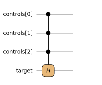
最初に、既定値のCLEAN_ANCILLA_TOFFOLIで推定します。このmodelでは、3個の制御条件の論理積を2個のclean ancillaへ計算し、controlled-Hadamardの適用後に元へ戻します。
decomposed_control_estimate = three_controlled_hadamard.estimate_resources()

print("分解後の総ゲート数:", decomposed_control_estimate.gates.total)
print("分解後のToffoliゲート数:", decomposed_control_estimate.gates.toffoli)
print(
    "分解で使うclean ancilla数:",
    decomposed_control_estimate.width.clean_ancilla_qubits,
)

assert decomposed_control_estimate.gates.total - 5 == 0
assert decomposed_control_estimate.gates.toffoli - 4 == 0
assert decomposed_control_estimate.width.clean_ancilla_qubits - 2 == 0
assert decomposed_control_estimate.qubits - 6 == 0
分解後の総ゲート数: 5
分解後のToffoliゲート数: 4
分解で使うclean ancilla数: 2
4個のToffoliゲートで論理積の計算とuncomputationを行うため、総ゲート数はcontrolled-Hadamardと合わせて5です。
次に、ABSTRACTを指定します。このmodelでは、controlled-Hadamardを分解せずに1個の多制御演算として数え、分解用ancillaを追加しません。
abstract_control_estimate = three_controlled_hadamard.estimate_resources(
    control_decomposition=qmc.ControlDecomposition.ABSTRACT,
)

print("ABSTRACTでの総ゲート数:", abstract_control_estimate.gates.total)
print(
    "ABSTRACTでのclean ancilla数:",
    abstract_control_estimate.width.clean_ancilla_qubits,
)

assert abstract_control_estimate.gates.total - 1 == 0
assert abstract_control_estimate.width.clean_ancilla_qubits - 0 == 0
assert abstract_control_estimate.qubits - 4 == 0
ABSTRACTでの総ゲート数: 1
ABSTRACTでのclean ancilla数: 0
以下では、Toffoliゲートとclean ancillaを使った分解を手書きし、総ゲート数、Toffoli数、深さ、ピーク幅がCLEAN_ANCILLA_TOFFOLIの推定結果と一致することを確認します。
@qmc.qkernel
def three_controlled_hadamard_manually() -> qmc.Qubit:
    """Apply a manually decomposed three-controlled Hadamard gate."""
    controls = qmc.qubit_array(3, "controls")
    target = qmc.qubit("target")
    ancillae = qmc.qubit_array(2, "ancillae")

    controls[0], controls[1], ancillae[0] = qmc.ccx(
        controls[0],
        controls[1],
        ancillae[0],
    )
    controls[2], ancillae[0], ancillae[1] = qmc.ccx(
        controls[2],
        ancillae[0],
        ancillae[1],
    )
    ancillae[1], target = qmc.control(qmc.h)(ancillae[1], target)
    controls[2], ancillae[0], ancillae[1] = qmc.ccx(
        controls[2],
        ancillae[0],
        ancillae[1],
    )
    controls[0], controls[1], ancillae[0] = qmc.ccx(
        controls[0],
        controls[1],
        ancillae[0],
    )
    return target


three_controlled_hadamard_manually.draw()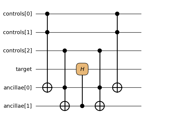
分解を手書きした量子カーネルを推定し、CLEAN_ANCILLA_TOFFOLIの結果と比較します。
manual_control_estimate = three_controlled_hadamard_manually.estimate_resources()

print("手書き分解の総ゲート数:", manual_control_estimate.gates.total)
print("手書き分解のToffoliゲート数:", manual_control_estimate.gates.toffoli)
print(
    "手書き分解で確保する量子ビット数:", manual_control_estimate.width.allocated_qubits
)
print(
    "手書き分解のclean_ancilla_qubits:",
    manual_control_estimate.width.clean_ancilla_qubits,
)

assert (
    manual_control_estimate.gates.total - decomposed_control_estimate.gates.total == 0
)
assert (
    manual_control_estimate.gates.toffoli - decomposed_control_estimate.gates.toffoli
    == 0
)
assert manual_control_estimate.qubits - decomposed_control_estimate.qubits == 0
assert (
    manual_control_estimate.depth.depth - decomposed_control_estimate.depth.depth == 0
)
assert manual_control_estimate.width.allocated_qubits - 6 == 0
assert manual_control_estimate.width.clean_ancilla_qubits - 0 == 0
手書き分解の総ゲート数: 5
手書き分解のToffoliゲート数: 4
手書き分解で確保する量子ビット数: 6
手書き分解のclean_ancilla_qubits: 0
CLEAN_ANCILLA_TOFFOLIの推定結果と分解を手書きした量子カーネルは、どちらも4個のToffoliゲートと1個のcontrolled-Hadamardを使い、ピーク幅は6です。手書きの量子カーネルでは、2個のancillaを量子カーネル内で明示的に確保したため、allocated_qubitsに含まれます。一方、CLEAN_ANCILLA_TOFFOLIでは、元の量子カーネルが確保する4個とは別に、推定modelが追加する2個をclean_ancilla_qubitsとして数えます。
4.2 unknown resource policy
costを指定していないOracleを含む量子カーネルを推定する場合は、unknown_policyで未知部分の扱いを選びます。既定値はERRORで、未知のcostを暗黙に0とせず、ValueErrorとします。
unpriced_step = qmc.Oracle(
    "unpriced_step",
    num_qubits=1,
)


@qmc.qkernel
def with_unpriced_oracle() -> qmc.Qubit:
    """Invoke an Oracle without a resource cost."""
    target = qmc.qubit("target")
    (target,) = unpriced_step(target)
    return target


with_unpriced_oracle.draw()
まず、unknown_policyを指定せず、既定値のERRORで推定します。costのないOracleを暗黙にコスト0とは扱わず、ValueErrorとします。
try:
    with_unpriced_oracle.estimate_resources()
except ValueError as error:
    print(error)
    assert "no body or opaque cost" in str(error)
else:
    raise AssertionError("An unpriced Oracle must fail by default.")
Cannot estimate resources for callable 'unpriced_step': no body or opaque cost is available.
未知部分があってもエラーにせずリソース推定を続けたい場合は、OPAQUE_CALLまたはZERO_WITH_WARNINGを明示的に選べます。
OPAQUE_CALLは、未知部分のゲート数や幅を推測せず、名前付きcallとqueryを1回ずつ記録し、具体的なcostがないことをassumptionsへ記録します。
opaque_call_estimate = with_unpriced_oracle.estimate_resources(
    unknown_policy=qmc.UnknownResourcePolicy.OPAQUE_CALL,
)

print("opaque callのゲート数:", opaque_call_estimate.gates.total)
print("opaque calls:", opaque_call_estimate.calls.calls_by_name)
print("opaque queries:", opaque_call_estimate.calls.queries_by_name)

assert opaque_call_estimate.gates.total - 0 == 0
assert opaque_call_estimate.calls.calls_by_name == {"unpriced_step": 1}
assert opaque_call_estimate.calls.queries_by_name == {"unpriced_step": 1}
assert any(
    assumption.message
    == "unknown callable is recorded as an opaque call without a declared resource cost"
    and assumption.source == "unpriced_step"
    for assumption in opaque_call_estimate.assumptions
)
assert opaque_call_estimate.quality is qmc.EstimateQuality.UNKNOWN
opaque callのゲート数: 0
opaque calls: {'unpriced_step': 1}
opaque queries: {'unpriced_step': 1}
ZERO_WITH_WARNINGは、未知部分を0と仮定して推定を続け、その仮定を結果のassumptionsへ記録します。ここでwarningはPythonのwarningとして出力されるのではなく、.assumptionsフィールドに記録されることに注意してください。
zero_warning_estimate = with_unpriced_oracle.estimate_resources(
    unknown_policy=qmc.UnknownResourcePolicy.ZERO_WITH_WARNING,
)

print("zero-with-warningのゲート数:", zero_warning_estimate.gates.total)
print("zero-with-warningのassumptions:")
for assumption in zero_warning_estimate.assumptions:
    print(f"- {assumption.message} (source: {assumption.source})")

assert zero_warning_estimate.gates.total - 0 == 0
assert zero_warning_estimate.calls.calls_by_name == {}
assert zero_warning_estimate.calls.queries_by_name == {}
assert any(
    assumption.message == "unknown callable counted as zero resources"
    and assumption.source == "unpriced_step"
    for assumption in zero_warning_estimate.assumptions
)
assert zero_warning_estimate.quality is qmc.EstimateQuality.UNKNOWN
zero-with-warningのゲート数: 0
zero-with-warningのassumptions:
- unknown callable counted as zero resources (source: unpriced_step)
| policy | 未知部分の扱い |
|---|---|
ERROR | 既定値。costのないOracleをValueErrorとする |
OPAQUE_CALL | ゲートのcostを推測せず、名前付きcallとqueryを1回ずつ記録し、その理由をassumptionsへ記録する |
ZERO_WITH_WARNING | 未知部分を0と仮定し、その仮定をassumptionsへ記録する |
OPAQUE_CALLとZERO_WITH_WARNINGでゲート数が0でも、未知部分にゲートがないという意味ではありません。どちらもqualityはUNKNOWNとなり、推定できなかった部分があることを示します。unknown_policyが影響するのはcostを指定していないOracleです。第3章のように固定costまたはcallbackを指定したOracleでは、そのcostが使われます。このため、明示的に0として扱いたい場合はcostへ0を指定してください。
5. 推定結果の確かさを確認する
リソースの数値だけでなく、推定結果のderivation、quality、approximationも確認すると、その数値がどのように計算されたかが分かります。この三つは、それぞれ異なる問いに答える独立した項目です。
5.1 三つの独立した軸
| 項目 | 確認できること | 値 |
|---|---|---|
derivation | 推定値をどのように求めたか | STRUCTURAL / MODELED |
quality | 推定結果に含まれる曖昧さ | EXACT / CONSERVATIVE / UNKNOWN |
approximation | 推定器が認識している数学的な近似が含まれるか | EXACT / APPROXIMATE |
derivation=STRUCTURALは、定義された量子カーネルと選択した分解規則を再帰的に実際に数えたことを表します。MODELEDは、Oracleへ指定したcostや、costのないOracleに対して選択したunknown_policyを使って数値を求めたことを表します。
quality=EXACTは、選択した分解規則や宣言したcostを含む推定対象に対して、推定値が一致することを表します。CONSERVATIVEは過小評価しない安全側の値、UNKNOWNはEXACTともCONSERVATIVEとも確認できない値です。
qualityがCONSERVATIVEまたはUNKNOWNである場合、その理由は必ずassumptionsにも含まれます。複数の理由が有効ならすべて保持され、より弱いqualityが全体の値として表示されても、それ以前の理由は失われません。逆に、assumptionsがあるだけでqualityがEXACTから下がるとは限りません。
approximationは、数値の数え方ではなく、推定結果に理想的な数学的操作に対する既知の近似が含まれているかを表します。
bell_pair:STRUCTURAL / EXACT / EXACT
bell_pairでは、推定器が定義した量子カーネルから、曖昧さなくcostを正確に数えています。また、推定器が認識する数学的な近似も含まれません。
print("derivation:", bell_estimate.derivation.value)
print("quality:", bell_estimate.quality.value)
print("approximation:", bell_estimate.approximation.value)

assert bell_estimate.derivation is qmc.EstimateDerivation.STRUCTURAL
assert bell_estimate.quality is qmc.EstimateQuality.EXACT
assert bell_estimate.approximation is qmc.ApproximationStatus.EXACT
derivation: structural
quality: exact
approximation: exact
固定costのOracle:MODELED / EXACT / EXACT
fixed_lookupの内部構造は見えませんが、利用者が1回分のcostを指定しています。そのためderivationはMODELEDで、指定したbase costに対するqualityはEXACTです。
print("derivation:", fixed_oracle_estimate.derivation.value)
print("quality:", fixed_oracle_estimate.quality.value)
print("approximation:", fixed_oracle_estimate.approximation.value)

assert fixed_oracle_estimate.derivation is qmc.EstimateDerivation.MODELED
assert fixed_oracle_estimate.quality is qmc.EstimateQuality.EXACT
assert fixed_oracle_estimate.approximation is qmc.ApproximationStatus.EXACT
derivation: modeled
quality: exact
approximation: exact
clean ancillaを使うcontrol分解:STRUCTURAL / CONSERVATIVE / EXACT
CLEAN_ANCILLA_TOFFOLIでは、定義した量子カーネル内の制御演算を固定のalgorithmic modelで分解し、安全側のcostを求めます。これは数学的な近似ではないため、approximationはEXACTです。
print("derivation:", decomposed_control_estimate.derivation.value)
print("quality:", decomposed_control_estimate.quality.value)
print("approximation:", decomposed_control_estimate.approximation.value)

assert decomposed_control_estimate.derivation is qmc.EstimateDerivation.STRUCTURAL
assert decomposed_control_estimate.quality is qmc.EstimateQuality.CONSERVATIVE
assert decomposed_control_estimate.approximation is qmc.ApproximationStatus.EXACT
derivation: structural
quality: conservative
approximation: exact
costのないOracle:MODELED / UNKNOWN / EXACT
OPAQUE_CALLは、costのないOracleを名前付きcall/queryとして記録し、具体的なcostがないことをassumptionsへ記録します。具体的なゲートのcostとの関係は分からないためqualityはUNKNOWNですが、推定器が認識する数学的な近似が追加されるわけではありません。
print("derivation:", opaque_call_estimate.derivation.value)
print("quality:", opaque_call_estimate.quality.value)
print("approximation:", opaque_call_estimate.approximation.value)

assert opaque_call_estimate.derivation is qmc.EstimateDerivation.MODELED
assert opaque_call_estimate.quality is qmc.EstimateQuality.UNKNOWN
assert opaque_call_estimate.approximation is qmc.ApproximationStatus.EXACT
derivation: modeled
quality: unknown
approximation: exact
非可換なPauli項の時間発展:STRUCTURAL / EXACT / APPROXIMATE
最後に、1個の量子ビットへ、互いに可換ではないX項とZ項の和による時間発展を適用します。理想的なHamiltonianの時間発展を1次のLie–Trotter積公式で近似し、そのときに使うリソースを推定します。
@qmc.qkernel
def one_qubit_pauli_evolution(
    hamiltonian: qmc.Observable,
    time: qmc.Float,
) -> qmc.Vector[qmc.Qubit]:
    """Apply one Pauli-sum evolution to a single qubit."""
    target = qmc.qubit_array(1, "target")
return qmc.pauli_evolve(target, hamiltonian, time)Hamiltonianと時間をinputsで具体化して推定し、三つのmetadataを確認します。
noncommuting_evolution_estimate = one_qubit_pauli_evolution.estimate_resources(
    inputs={
        "hamiltonian": qmo.X(0) + qmo.Z(0),
        "time": 0.25,
    },
)

print("derivation:", noncommuting_evolution_estimate.derivation.value)
print("quality:", noncommuting_evolution_estimate.quality.value)
print("approximation:", noncommuting_evolution_estimate.approximation.value)

assert noncommuting_evolution_estimate.derivation is qmc.EstimateDerivation.STRUCTURAL
assert noncommuting_evolution_estimate.quality is qmc.EstimateQuality.EXACT
assert (
    noncommuting_evolution_estimate.approximation is qmc.ApproximationStatus.APPROXIMATE
)
derivation: structural
quality: exact
approximation: approximate
この例では、選択された1次のLie–Trotter積公式に含まれるゲートを正確に数えるため、quality=EXACTです。一方、その積公式自体は理想的な時間発展の近似なので、approximation=APPROXIMATEになります。
5.2 assumptions
assumptionsには、三つの項目だけでは表せない具体的な前提や理由が入ります。これには、CONSERVATIVEまたはUNKNOWNとなった理由、モデル上の仮定、リソース式の簡約に使った未具体化の有効な入力条件が含まれます。リソース推定器は、量子カーネルの入力型、量子ビット配列を含む配列のshape、配列要素へのアクセス、viewの範囲などから有効な入力条件を導ける場合、その条件が成り立つ範囲でリソース式を簡約し、未具体化の条件をassumptionsに残します。各要素は、説明文のmessageと、原因となった演算などを示すsourceを持ちます。有効な入力条件は式の適用範囲を示すものであり、それだけでqualityがEXACTから下がるわけではありません。上のGHZ例では、CXの列を実行した後に各量子ビットが準備できる時刻が異なります。現在の推定器は、このループと後続のmeasure(qubits)との依存を、量子ビットごとの完了時刻ではなくループ全体の最長時間を使って安全側に扱うため、早く準備できた量子ビットの測定を必要以上に遅く見積もる可能性があります。そのためqualityはCONSERVATIVEになり、この理由もassumptionsに記録されます。このGHZでは最後に準備できる量子ビットが実際の全体の深さも決めるので、推定された深さn + 1は実際のスケジュールと一致します。これは有効な入力条件を使った簡約とは別の理由です。
ZERO_WITH_WARNINGを使った推定結果には、costのないOracleを0として数えたことが記録されます。
print("unknown-cost assumptions:")
for assumption in zero_warning_estimate.assumptions:
    print(f"- {assumption.message} (source: {assumption.source})")

assert any(
    assumption.message == "unknown callable counted as zero resources"
    for assumption in zero_warning_estimate.assumptions
)
unknown-cost assumptions:
- unknown callable counted as zero resources (source: unpriced_step)
非可換なPauli項の時間発展には、数学的な近似が含まれていることが記録されます。
print("Pauli-evolution assumptions:")
for assumption in noncommuting_evolution_estimate.assumptions:
    print(f"- {assumption.message} (source: {assumption.source})")

assert any(
    "first-order Lie-Trotter" in assumption.message
    for assumption in noncommuting_evolution_estimate.assumptions
)
Pauli-evolution assumptions:
- Noncommuting Pauli terms are counted as one first-order Lie-Trotter product-formula step in Hamiltonian term order. (source: PauliEvolveOp)
Appendix: ResourceEstimateの全フィールド一覧
リソース項目には、具体的な整数だけでなく、問題サイズに依存するSymPyの式が入る場合があります。通常は第2章で扱った代表的な項目を確認すれば十分ですが、ここでは公開されている全フィールドを参照用にまとめます。
ResourceEstimate
| フィールド | 内容 |
|---|---|
width | 論理量子ビット幅とancillaの推定値 |
gates | 論理ゲート数の推定値 |
measurements | 測定イベント数の推定値 |
resets | リセット数の推定値 |
depth | 論理的な深さの推定値 |
calls | 名前別に記録したopaque call/queryの回数 |
parameters | 未具体化のシンボリックなパラメータ名とSymPy symbolの対応 |
assumptions | 推定時の前提と理由。非EXACTの理由、モデル上の仮定、式の簡約に使った未具体化の有効な入力条件を含み、各要素はmessageとsourceを持つ |
derivation | 量子カーネルそのものから導き出されるSTRUCTURALか、cost/policyを使ったMODELEDか |
quality | 推定結果に含まれる曖昧さについてEXACT、CONSERVATIVE、UNKNOWNのどれか |
approximation | 認識されている数学的な近似がEXACTかAPPROXIMATEか |
control_decomposition | 推定に使用したcoherent controlの分解方法 |
trace | trace=Trueを指定した場合だけ保持する診断用tree。通常はNone |
Width
estimate.widthはWidthResourcesです。
| フィールド | 内容 |
|---|---|
input_qubits | 呼び出し側から渡される量子ビット数 |
allocated_qubits | 本体にある静的な確保場所の量子ビット数 |
clean_ancilla_qubits | 初期状態` |
dirty_ancilla_qubits | 任意の初期状態を借り、使用後に元へ戻すancillaのpeak需要 |
peak_qubits | 実行中に同時にliveとなる論理量子ビットの最大数 |
allocated_qubits、clean_ancilla_qubits、dirty_ancilla_qubitsは別々の分類です。clean/dirty ancillaがallocated_qubitsの内訳という意味ではありません。
ゲート
estimate.gatesはGateResourcesです。
| フィールド | 内容 |
|---|---|
total | 測定とリセットを含まない論理ゲートの総数 |
single_qubit | 1個の量子ビットへ作用するゲート数 |
two_qubit | 2個の量子ビットへ作用するゲート数 |
multi_qubit | 3個以上の量子ビットへ作用するゲート数 |
clifford | Cliffordゲート数 |
rotation | RX、RY、RZ、P、CP、RZZなどの回転ゲート数 |
t | T/T-daggerゲート数 |
toffoli | Toffoliゲート数 |
non_clifford | non-Cliffordゲート数 |
single_qubit、two_qubit、multi_qubitは作用する量子ビット数による分類です。clifford以降はゲートの種類による分類であり、二つの分類は重なります。すべてのフィールドを足し合わせるものではありません。また、Oracleへ一部のcostだけを指定した場合は、作用する量子ビット数ごとの内訳の和がtotalと一致しないことがあります。
測定・リセット
| フィールド | 内容 |
|---|---|
estimate.measurements.total | 量子ビットごとの測定イベント数。N個の量子ビットを測定するとN増える |
estimate.resets.total | 量子ビットごとの明示的なリセット数 |
測定とリセットはgates.totalには含まれません。
深さ
estimate.depthはDepthResourcesです。
| フィールド | 内容 |
|---|---|
depth | ゲート、測定、リセットがレイヤー数に寄与する全体のクリティカルパスの長さ |
gate_depth | ゲートだけがレイヤー数に寄与する深さ |
measurement_depth | 測定だけがレイヤー数に寄与する深さ |
reset_depth | リセットだけがレイヤー数に寄与する深さ |
clifford_depth | Cliffordゲートだけがレイヤー数に寄与する深さ |
rotation_depth | 回転ゲートだけがレイヤー数に寄与する深さ |
t_depth | T/T-daggerゲートだけがレイヤー数に寄与する深さ |
toffoli_depth | Toffoliゲートだけがレイヤー数に寄与する深さ |
non_clifford_depth | non-Cliffordゲートだけがレイヤー数に寄与する深さ |
種類別の深さでも、対象外の演算はレイヤー数を増やさないだけで、依存関係と順序は引き続き保たれます。これらを足してもdepth.depthにはなりません。
Calls / queries
estimate.callsはCallResourcesです。
| フィールド | 内容 |
|---|---|
calls_by_name | 本体を展開せずに残した、またはcostで明示した名前付きcallの回数 |
queries_by_name | 名前ごとに明示またはmodel化したalgorithmicなOracle query回数 |
本体を解析できる通常の量子カーネルcallは再帰的に展開されるため、calls_by_nameには残りません。OPAQUE_CALLでは情報がない場合の規則として両方へ1を記録しますが、callとqueryは異なる意味を持つフィールドです。
Convenience aliases
次のpropertyは、よく使うフィールドへ短くアクセスするためのaliasまたは計算値です。
| property | 対応する値 |
|---|---|
estimate.qubits | estimate.width.peak_qubits |
estimate.width.circuit_qubits | input_qubits + allocated_qubits + clean_ancilla_qubits + dirty_ancilla_qubits |
estimate.circuit_qubits | estimate.width.circuit_qubits |
estimate.gates.t_gates | estimate.gates.t |
estimate.gates.clifford_gates | estimate.gates.clifford |
estimate.gates.rotation_gates | estimate.gates.rotation |
estimate.calls.oracle_calls | estimate.calls.calls_by_name |
estimate.calls.oracle_queries | estimate.calls.queries_by_name |
まとめ
estimate_resources()を使うと、特定のengine向けにtranspileする前のアルゴリズムレベルのリソースを推定できます。パラメータ付きの量子カーネルはシンボリックに推定でき、推定時に構造を具体化する場合は
inputs、得られた式を評価する場合は.substitute()を使います。本体を持たないOracleには、固定costまたはcallbackで1回分のbase costを設定できます。
derivation、quality、approximation、assumptionsを確認することで、リソース推定結果がどのように計算されたかを確認することができます。