Using OMMX Quantum Benchmarks (1): Implementing and Benchmarking Quantum Algorithms with Qamomile

Tags: integration optimization variational

This tutorial shows how to run a Qamomile quantum algorithm on a problem from a public benchmark dataset and compare its solution quality with a classical solver in the same workflow.

Goal. Build a QAOA solver in Qamomile, run it on a Low Autocorrelation Binary Sequences (LABS) instance loaded from the OMMX Quantum Benchmarks dataset, and compare the result with the classical SCIP solver accessed through the ommx-pyscipopt-adapter. Because both the QAOA path and the SCIP path consume the same ommx.v1.Instance, the main difference is the algorithm itself. This makes the comparison direct.

# Install the additional packages used in this tutorial.
# !pip install qamomile ommx-quantum-benchmarks ommx-pyscipopt-adapter

import os
import time

# `ommx-quantum-benchmarks` uses `minto` internally and, by default,
# `minto` prints a host-environment dump (Python version, virtualenv
# path, etc.) at experiment start. Suppress it so the rendered
# notebook outputs do not leak local-machine details.
os.environ["MINTO_TESTING"] = "true"

import matplotlib.pyplot as plt
import numpy as np
import ommx.v1
import ommx_pyscipopt_adapter
from ommx_quantum_benchmarks.qoblib import Labs
from qiskit_aer import AerSimulator
from qiskit_aer.primitives import EstimatorV2
from scipy.optimize import minimize

import qamomile.circuit as qmc
import qamomile.observable as qm_o
from qamomile.optimization.binary_model import BinaryModel, VarType
from qamomile.qiskit import QiskitTranspiler
from qamomile.qiskit.transpiler import QiskitExecutor

What is OMMX Quantum Benchmarks?¶

OMMX (Open Mathematical prograMming eXchange) is a data format for exchanging mathematical optimization problems across tools. Its ommx.v1.Instance stores the objective, constraints, and decision-variable metadata.

OMMX Quantum Benchmarks is a curated collection of optimization benchmark instances distributed in this ommx.v1.Instance format. The first dataset shipped is QOBLIB (Quantum Optimization Benchmarking Library) arXiv:2504.03832, which contains nine problem families used in the recent quantum-optimization literature, including LABS, Market Split, Independent Set, and Steiner-tree packing.

Because each benchmark instance is represented as an ommx.v1.Instance, any Qamomile workflow that accepts ommx.v1.Instance, including QAOAConverter, can consume these problems without writing any extra code. In addition, a reference solution is provided in the ommx.v1.Solution format and can be used to evaluate benchmark results. The same Instance can also be passed to classical OMMX adapters such as ommx-pyscipopt-adapter, so one problem definition can support both quantum and classical workflows.

Problem: Low Autocorrelation Binary Sequences (LABS)¶

LABS asks for a binary sequence $\boldsymbol{s} = (s_0, s_1, \dots, s_{n-1}) \in \{-1, +1\}^n$ whose off-diagonal autocorrelations

c_k(\boldsymbol{s}) = \sum_{i=0}^{n-k-1} s_i \, s_{i+k}, \qquad k = 1, 2, \dots, n-1

(1)

are as close to zero as possible. The benchmark objective is the sum of squared autocorrelations

E(\boldsymbol{s}) = \sum_{k=1}^{n-1} c_k(\boldsymbol{s})^2,

(2)

which we want to minimize. LABS is NP-hard and has long served as a stress test for both classical and quantum heuristics.

Loading a LABS instance¶

Labs exposes two models: "integer" (uses integer decision variables for $c_k$ plus the constraints that tie them to $\boldsymbol{s}$ ) and "quadratic_unconstrained" (a QUBO reformulation that introduces auxiliary binary variables $z_{i,k}$ encoding the products $x_i x_{i+k+1}$ via a quadratic penalty). The QUBO form is the natural target for QAOA, so we use it here.

dataset = Labs()
print(f"Dataset:           {dataset.name}")
print(f"Available models:  {dataset.model_names}")
print(f"Instance count:    {len(dataset.available_instances['quadratic_unconstrained'])}")
print(f"First 5 instances: {dataset.available_instances['quadratic_unconstrained'][:5]}")

Dataset:           02_labs
Available models:  ['integer', 'quadratic_unconstrained']
Instance count:    99
First 5 instances: ['labs002', 'labs003', 'labs004', 'labs005', 'labs006']

We pick labs005, the $n=5$ instance. The QUBO reformulation uses $n + n(n-1) = 25$ binary variables (5 sequence bits $x_i$ plus $n(n-1) = 20$ auxiliary $z_{i,k}$ bits). After Instance.to_qubo() folds the penalty terms into the objective and inactive variables are pruned, this becomes a 15-qubit problem: small enough to simulate locally, but large enough that QAOA is non-trivial.

instance, reference_solution = dataset("quadratic_unconstrained", "labs005")
n = 5

print(f"OMMX variables:    {instance.num_variables}")
print(f"OMMX constraints:  {instance.num_constraints}")
print(f"Reference E(s):    {reference_solution.objective}")
print(f"Reference feasible: {reference_solution.feasible}")

OMMX variables:    25
OMMX constraints:  0
Reference E(s):    2.0
Reference feasible: True

The bundled reference solution gives the known optimum $E^\star = 2$ for $n=5$ . We will compare both QAOA and SCIP against this value.

Algorithm: QAOA¶

Rather than use the high-level QAOAConverter, we build the QAOA workflow from scratch with @qkernel, following the recipe in QAOA for MaxCut: Building the Circuit from Scratch. Refer to that tutorial for the gate-by-gate derivation; here we focus on the implementation.

Spin model from the OMMX instance¶

Instance.to_qubo() converts the penalty-form ommx.v1.Instance into a QUBO. We then wrap it in a BinaryModel and switch to the spin (-1/+1) domain, which is what the QAOA cost layer expects. We also normalize the coefficients so the energy scale stays comparable across runs.

# `Instance.to_qubo()` mutates the instance (it absorbs constraints into
# the objective via the penalty method). Round-trip through bytes to keep
# the caller's instance untouched.
instance_for_qubo = ommx.v1.Instance.from_bytes(instance.to_bytes())
qubo, qubo_constant = instance_for_qubo.to_qubo()
spin_model = (
    BinaryModel.from_qubo(qubo, qubo_constant)
    .change_vartype(VarType.SPIN)
    .normalize_by_abs_max()
)
print(f"QAOA qubits: {spin_model.num_bits}")

QAOA qubits: 15

Cost Hamiltonian¶

To use the exact expectation value rather than a shot estimate for the optimization, we build the Ising cost Hamiltonian directly from the spin-model coefficients: $Z_i$ terms for the linear part and $Z_i Z_j$ terms for the quadratic part.

cost_hamiltonian = qm_o.Hamiltonian()
for i, hi in spin_model.linear.items():
    if abs(hi) > 1e-12:
        cost_hamiltonian.add_term((qm_o.PauliOperator(qm_o.Pauli.Z, i),), hi)
for (i, j), Jij in spin_model.quad.items():
    if abs(Jij) > 1e-12:
        cost_hamiltonian.add_term(
            (qm_o.PauliOperator(qm_o.Pauli.Z, i), qm_o.PauliOperator(qm_o.Pauli.Z, j)),
            Jij,
        )
cost_hamiltonian.constant = spin_model.constant

QAOA qkernels¶

The ansatz uses three small qkernels: a uniform superposition, a cost layer, and a mixer layer. We compose them into a state-preparation qkernel qaoa_state, then wrap it twice: once with qmc.expval to get an expectation-value qkernel for the optimizer, and once with qmc.measure to get a sampling qkernel for the final shot histogram.

@qmc.qkernel
def superposition(n: qmc.UInt) -> qmc.Vector[qmc.Qubit]:
    q = qmc.qubit_array(n, name="q")
    for i in qmc.range(n):
        q[i] = qmc.h(q[i])
    return q


@qmc.qkernel
def cost_layer(
    quad: qmc.Dict[qmc.Tuple[qmc.UInt, qmc.UInt], qmc.Float],
    linear: qmc.Dict[qmc.UInt, qmc.Float],
    q: qmc.Vector[qmc.Qubit],
    gamma: qmc.Float,
) -> qmc.Vector[qmc.Qubit]:
    for (i, j), Jij in quad.items():
        q[i], q[j] = qmc.rzz(q[i], q[j], angle=Jij * gamma)
    for i, hi in linear.items():
        q[i] = qmc.rz(q[i], angle=hi * gamma)
    return q


@qmc.qkernel
def mixer_layer(
    q: qmc.Vector[qmc.Qubit],
    beta: qmc.Float,
) -> qmc.Vector[qmc.Qubit]:
    n = q.shape[0]
    for i in qmc.range(n):
        q[i] = qmc.rx(q[i], angle=2.0 * beta)
    return q


@qmc.qkernel
def qaoa_state(
    p: qmc.UInt,
    quad: qmc.Dict[qmc.Tuple[qmc.UInt, qmc.UInt], qmc.Float],
    linear: qmc.Dict[qmc.UInt, qmc.Float],
    n: qmc.UInt,
    gammas: qmc.Vector[qmc.Float],
    betas: qmc.Vector[qmc.Float],
) -> qmc.Vector[qmc.Qubit]:
    q = superposition(n)
    for layer in qmc.range(p):
        q = cost_layer(quad, linear, q, gammas[layer])
        q = mixer_layer(q, betas[layer])
    return q


@qmc.qkernel
def qaoa_expval(
    p: qmc.UInt,
    quad: qmc.Dict[qmc.Tuple[qmc.UInt, qmc.UInt], qmc.Float],
    linear: qmc.Dict[qmc.UInt, qmc.Float],
    n: qmc.UInt,
    gammas: qmc.Vector[qmc.Float],
    betas: qmc.Vector[qmc.Float],
    H: qmc.Observable,
) -> qmc.Float:
    q = qaoa_state(p, quad, linear, n, gammas, betas)
    return qmc.expval(q, H)


@qmc.qkernel
def qaoa_sampling(
    p: qmc.UInt,
    quad: qmc.Dict[qmc.Tuple[qmc.UInt, qmc.UInt], qmc.Float],
    linear: qmc.Dict[qmc.UInt, qmc.Float],
    n: qmc.UInt,
    gammas: qmc.Vector[qmc.Float],
    betas: qmc.Vector[qmc.Float],
) -> qmc.Vector[qmc.Bit]:
    q = qaoa_state(p, quad, linear, n, gammas, betas)
    return qmc.measure(q)

Transpile and optimize¶

Transpile both kernels with $p = 3$ . The expectation-value executable is used for the optimization; the sampling executable is used later for the final shot histogram. We feed the optimizer the exact expectation value of the cost Hamiltonian via Aer’s EstimatorV2 primitive, which keeps the BFGS finite-difference gradient free of sampling noise. We seed NumPy so the parameter trajectory is reproducible.

p = 3
transpiler = QiskitTranspiler()
expval_executable = transpiler.transpile(
    qaoa_expval,
    bindings={
        "p": p,
        "quad": spin_model.quad,
        "linear": spin_model.linear,
        "n": spin_model.num_bits,
        "H": cost_hamiltonian,
    },
    parameters=["gammas", "betas"],
)
sampling_executable = transpiler.transpile(
    qaoa_sampling,
    bindings={
        "p": p,
        "quad": spin_model.quad,
        "linear": spin_model.linear,
        "n": spin_model.num_bits,
    },
    parameters=["gammas", "betas"],
)

SEED = 42
executor = QiskitExecutor(
    backend=AerSimulator(seed_simulator=SEED, max_parallel_threads=1),
    estimator=EstimatorV2(),
)

docs_test_mode = os.environ.get("QAMOMILE_DOCS_TEST") == "1"
maxiter = 5 if docs_test_mode else 50

rng = np.random.default_rng(SEED)
initial_params = rng.uniform(0, np.pi, 2 * p)

cost_history: list[float] = []


def cost_fn(params: np.ndarray) -> float:
    """Return the exact expectation value of the cost Hamiltonian at `params`."""
    gammas = list(params[:p])
    betas = list(params[p:])
    job = expval_executable.run(
        executor,
        bindings={"gammas": gammas, "betas": betas},
    )
    energy = job.result()
    cost_history.append(energy)
    return energy


t0 = time.perf_counter()
res = minimize(
    cost_fn,
    initial_params,
    method="BFGS",
    options={"maxiter": maxiter},
)
qaoa_optimize_time = time.perf_counter() - t0

print(f"Optimized expectation value (normalized): {res.fun:.4f}")
print(f"Function evaluations:                     {res.nfev}")
print(f"Wall time:                                {qaoa_optimize_time:.2f} s")

Optimized expectation value (normalized): 1.9622
Function evaluations:                     385
Wall time:                                4.31 s

plt.figure(figsize=(8, 4))
plt.plot(cost_history, color="#2696EB")
plt.xlabel("Iteration")
plt.ylabel("Expectation value (normalized)")
plt.title("QAOA Optimization Progress (LABS, n=5)")
plt.show()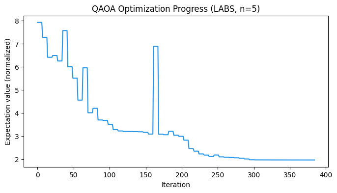

Final sampling¶

We sample once more with the optimized parameters and a larger shot count. Then we decode against the original ommx.v1.Instance, so the returned ommx.v1.SampleSet reports the original QUBO objective directly. In this QUBO formulation, samples whose auxiliary $z$ variables correctly encode the products $x_i x_{i+k+1}$ incur no penalty, and the objective equals the LABS energy $E(\boldsymbol{s}) = \sum_k c_k^2$ . Samples that violate the implicit $z = x_i x_{i+k+1}$ relation incur an additive penalty.

def evaluate_with_ommx(
    sample_result, spin_model: BinaryModel, ommx_instance: ommx.v1.Instance
) -> ommx.v1.SampleSet:
    """Decode SPIN samples, flip to BINARY, and evaluate against the OMMX instance."""
    spin_ss = spin_model.decode_from_sampleresult(sample_result)
    ommx_samples = ommx.v1.Samples({})
    next_id = 0
    for sample, occ in zip(spin_ss.samples, spin_ss.num_occurrences):
        if occ <= 0:
            continue
        # SPIN (+/-1) -> BINARY (0/1): x = (1 - s) / 2
        binary_state = {idx: (1 - val) // 2 for idx, val in sample.items()}
        sample_ids = list(range(next_id, next_id + occ))
        next_id += occ
        ommx_samples.append(
            sample_ids,
            ommx.v1.State({idx: float(val) for idx, val in binary_state.items()}),
        )
    return ommx_instance.evaluate_samples(ommx_samples)


gammas_opt = list(res.x[:p])
betas_opt = list(res.x[p:])
final_shots = 256 if docs_test_mode else 4096

final_result = sampling_executable.sample(
    executor,
    shots=final_shots,
    bindings={"gammas": gammas_opt, "betas": betas_opt},
).result()
qaoa_sample_set = evaluate_with_ommx(final_result, spin_model, instance)

qaoa_summary = qaoa_sample_set.summary
qaoa_best = qaoa_sample_set.best_feasible
qaoa_best_E = int(round(qaoa_best.objective))
ref_E = int(reference_solution.objective)

print(f"Shots:                {len(qaoa_summary)}")
print(f"QAOA best objective:  {qaoa_best_E}")
print(f"Reference E*:         {ref_E}")

Shots:                4096
QAOA best objective:  2
Reference E*:         2

Distribution of objective values¶

QAOA returns a distribution over bitstrings, not a single answer. The histogram below shows the QUBO objective of every shot at the optimized parameters. The red dashed line marks the reference optimum $E^\star$ . Samples on, or just to the right of, that line have $x$ values that minimize the LABS sum and $z$ values that correctly encode the products. Samples far to the right pay a penalty for inconsistent $z$ values.

objectives = qaoa_summary["objective"].to_numpy()

plt.figure(figsize=(8, 4))
plt.hist(objectives, bins=40, color="#2696EB", edgecolor="white")
plt.axvline(
    ref_E,
    color="red",
    linestyle="--",
    label=f"Reference $E^\\star$ = {ref_E}",
)
plt.xlabel("Objective value (QUBO energy)")
plt.ylabel("Frequency")
plt.title(f"QAOA Output Distribution (p={p}, shots={final_shots})")
plt.legend()
plt.show()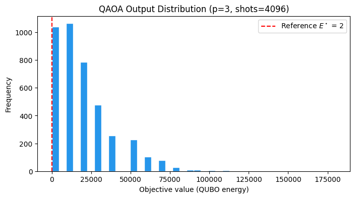

Classical baseline: SCIP via the OMMX adapter¶

SCIP is a branch-and-bound-based MILP/QUBO solver that can find the exact optimal solution. The same ommx.v1.Instance is consumed by ommx_pyscipopt_adapter.OMMXPySCIPOptAdapter.solve, which hands the problem to SCIP via PySCIPOpt and returns an ommx.v1.Solution evaluated against the original instance. Its .objective is therefore directly comparable to QAOA’s.

t0 = time.perf_counter()
scip_solution = ommx_pyscipopt_adapter.OMMXPySCIPOptAdapter.solve(instance)
scip_solve_time = time.perf_counter() - t0

scip_E = int(round(scip_solution.objective))
print(f"SCIP E(s):    {scip_E}")
print(f"SCIP feasible: {scip_solution.feasible}")
print(f"Wall time:    {scip_solve_time:.3f} s")

SCIP E(s):    2
SCIP feasible: True
Wall time:    0.124 s

Results comparison¶

SCIP returns a single optimum deterministically, while QAOA returns a distribution over bitstrings. We report QAOA’s best shot (the lowest-objective bitstring seen across all samples) and its hit rate on the reference optimum (the fraction of shots that achieved $E^\star$ ).

# Hit rate: fraction of shots that achieved the reference optimum.
hit_rate = float((qaoa_summary["objective"].round().astype(int) == ref_E).mean())

print(f"{'Solver':<22} {'E(s)':>8} {'Time (s)':>12}")
print("-" * 46)
print(f"{'Reference (bundled)':<22} {ref_E:>8} {'-':>12}")
print(f"{'SCIP (classical)':<22} {scip_E:>8} {scip_solve_time:>12.3f}")
print(f"{'QAOA (best shot)':<22} {qaoa_best_E:>8} {qaoa_optimize_time:>12.2f}")
print()
print(f"QAOA hit rate on E* = {ref_E}: {hit_rate:.1%}  ({final_shots} shots)")

Solver                     E(s)     Time (s)
----------------------------------------------
Reference (bundled)           2            -
SCIP (classical)              2        0.124
QAOA (best shot)              2         4.31

QAOA hit rate on E* = 2: 4.6%  (4096 shots)

Two observations make this benchmark meaningful:

Optimum. Both SCIP and the best QAOA shot reach the reference optimum $E^\star = 2$ , so QAOA is capable of finding the optimal sequence at $n = 5$ with only $p = 3$ .
Concentration. QAOA’s value lies in concentrating sampling probability on low-energy bitstrings. The hit rate above, together with the left tail of the histogram, is the quantitative version of that statement.

Note that the wall-time figures are only indicative. SCIP’s timing is just the solver’s runtime on the CPU, while the QAOA timing covers the full classical-quantum optimization loop on a state-vector simulator; both depend on the execution environment. A genuinely fair comparison would therefore require a more careful methodology. Either way, combining Qamomile with datasets like OMMX Quantum Benchmarks makes it easy to compare quantum algorithms and classical solvers across a variety of metrics.

Summary¶

In this tutorial we:

Loaded a LABS instance straight from the OMMX Quantum Benchmarks dataset as an ommx.v1.Instance.
Extracted the QUBO with Instance.to_qubo(), wrapped it in a BinaryModel, switched to the spin domain, and ran a hand-written QAOA ansatz (using @qkernel) against it through QiskitTranspiler + AerSimulator.
Compared the QAOA output (best shot, hit rate, sampling distribution) against SCIP via ommx_pyscipopt_adapter.OMMXPySCIPOptAdapter.solve on the same instance, plus the reference optimum bundled with the benchmark.

The pattern generalizes: any other QOBLIB dataset (Marketsplit, IndependentSet, Network, …) plugs into the same pipeline: load with the corresponding dataset class, extract the QUBO via Instance.to_qubo(), and reuse the same BinaryModel + QAOA ansatz + transpile loop. Larger instances will eventually outgrow local simulators, at which point the same executable can be re-targeted to other Qamomile quantum SDK integrations (QuriPartsTranspiler, CudaqTranspiler, …) or real hardware.