Your First Quantum Kernel

This chapter introduces the basic workflow for a first-time Qamomile user to define and run a quantum kernel. Note that this chapter does not dive into quantum computing fundamentals or quantum algorithm details.

What is Qamomile?¶

Qamomile is a quantum circuit SDK that lets you write quantum programs in Python, then run them on any supported quantum SDK (Qiskit, QuriParts, and more in plan). It uses a typed, symbolic approach: you write a Python function decorated with @qkernel, and Qamomile traces it into an intermediate representation that can be analyzed, visualized, and transpiled.

The core workflow is a simple pipeline:

@qkernel define  →  draw() / estimate_resources()  →  transpile()  →  sample() / run()  →  .result()

Define: Write a qkernel function with type annotations.
Inspect: Visualize the circuit with draw(), or estimate costs with estimate_resources().
Transpile: Transpile the qkernel into an executable for your chosen quantum SDK.
Execute: Run it with sample() (for measured bits) or run() (for expectation values).
Read results: Call .result() to get the output.

You do not need every step every time — use what fits your task.

Installation¶

For normal use:

pip install qamomile

In this tutorial we use Qiskit as the concrete quantum SDK. QuriParts is also supported, and more quantum SDKs will be added over time.

# Install the latest Qamomile through pip!
# !pip install qamomile

import math

import qamomile.circuit as qmc
from qamomile.qiskit import QiskitTranspiler

transpiler = QiskitTranspiler()

First QKernel: The Biased Coin¶

A QKernel is a Python function decorated with @qmc.qkernel. It describes a quantum circuit using typed handles and gate operations.

A handle is an “identifier” or “token” that indirectly references some resource or object.

Let’s build the simplest possible example: a single qubit rotated by an angle theta, then measured. Depending on theta, the qubit is biased toward 0 or 1 — like a biased coin.

@qmc.qkernel
def biased_coin(theta: qmc.Float) -> qmc.Bit:
    # Create a single qubit handle named "q"
    q = qmc.qubit(name="q")

    # Apply an RY rotation — this biases the qubit
    q = qmc.ry(q, theta)

    # Measure and return the result as a classical Bit
    return qmc.measure(q)

Key things to notice:

Type annotations are required. theta: qmc.Float says theta is a floating-point parameter. The return type qmc.Bit says this qkernel produces one classical bit.
qmc.qubit(name="q") creates a qubit handle. The name appears in circuit diagrams.
q = qmc.ry(q, theta) applies the RY gate and reassigns q. This reassignment is important — we will explain why shortly.
qmc.measure(q) measures the qubit state and returns a Bit.

Inspect Before Running¶

Before executing, you can inspect your qkernel. draw() shows the circuit diagram:

biased_coin.draw(theta=0.6)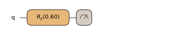

You can also check the cost of a qkernel before running it. estimate_resources() reports qubit count and gate counts:

est = biased_coin.estimate_resources()
print("qubits:", est.qubits)
print("total gates:", est.gates.total)

qubits: 1
total gates: 1

For this simple qkernel the numbers are concrete, but for parameterized qkernels they become symbolic SymPy expressions — we will explore this in detail in Tutorial 02.

The Execution Pipeline¶

Now let’s actually run this qkernel. The process has three steps:

Transpile: Transpile the qkernel into an executable object with a user-specific quantum SDK.
Execute: Call sample() to run it with specific parameter values.
Read results: Call .result() on the returned Job.

Here is the code, then we explain each part:

# Step 1: Transpile
# parameters=["theta"] tells the transpiler: "theta will be provided later,
# keep it as a sweepable parameter in the transpiled circuit."
exe = transpiler.transpile(biased_coin, parameters=["theta"])

# Step 2: Execute
# bindings={"theta": ...} provides the concrete value for theta.
# shots=256 means we run the circuit 256 times.
# The default executor (transpiler.executor()) uses a local simulator, but you can plug in
# your own custom executor (e.g., for real hardware or cloud services).
job = exe.sample(
    transpiler.executor(),
    shots=256,
    bindings={"theta": math.pi / 4},
)

# Step 3: Read results
# .result() blocks until the job completes and returns a SampleResult.
result = job.result()

print("sample results:", result.results)

sample results: [(0, 220), (1, 36)]

Let’s unpack the three concepts:

parameters=["theta"] at transpile time declares which qkernel inputs remain as tunable knobs in the transpiled program. Inputs not listed here must be provided via bindings at transpile time (we will see this in Tutorial 02).
bindings={"theta": math.pi / 4} at execution time fills in the concrete value for the parameter. The default executor uses a local simulator, but you may swap in a custom executor (e.g., real hardware or a cloud service) without changing your code.
.result(): sample() returns a Job object, not the result directly. Calling .result() waits for the job to finish and returns a SampleResult.

Reading `SampleResult`¶

result.results is a list[tuple[T, int]] where:

T is the measured output type (here, int — 0 or 1 for a Bit)
int is the count: how many times that outcome appeared

For example, [(0, 150), (1, 106)] means outcome 0 appeared 150 times and outcome 1 appeared 106 times out of 256 shots.

for value, count in result.results:
    print(f"  outcome={value}, count={count}")

  outcome=0, count=220
  outcome=1, count=36

SampleResult also provides convenience methods:

# Most common outcome
print("most common:", result.most_common(1))

# Probability distribution
print("probabilities:", result.probabilities())

most common: [(0, 220)]
probabilities: [(0, 0.859375), (1, 0.140625)]

Inspecting the Transpiled Circuit¶

to_circuit() transpiles a qkernel with all parameters bound and returns the quantum SDK-native circuit (e.g., a Qiskit QuantumCircuit). This is useful for debugging — you can see exactly how the circuit looks in the target SDK.

qiskit_circuit = transpiler.to_circuit(
    biased_coin,
    bindings={"theta": math.pi / 4},
)
print(qiskit_circuit)

     ┌─────────┐┌─┐
  q: ┤ Ry(π/4) ├┤M├
     └─────────┘└╥┘
c: 1/════════════╩═
                 0

Multi-Qubit Example¶

Let’s use more than one qubit. This example introduces two new things:

qubit_array(n) to allocate multiple qubits at once
cx() (the CNOT gate), a two-qubit gate that returns both handles

@qmc.qkernel
def two_qubit_demo() -> qmc.Vector[qmc.Bit]:
    q = qmc.qubit_array(2, name="q")

    q[0] = qmc.h(q[0])  # Apply H to q[0]
    q[0], q[1] = qmc.cx(q[0], q[1])  # Apply CNOT on q[0], q[1]

    return qmc.measure(q)

two_qubit_demo.draw()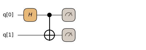

demo_result = (
    transpiler.transpile(two_qubit_demo)
    .sample(
        transpiler.executor(),
        shots=256,
    )
    .result()
)

for outcome, count in demo_result.results:
    print(f"  outcome={outcome}, count={count}")

  outcome=(1, 1), count=140
  outcome=(0, 0), count=116

Notice two patterns here:

qubit_array(2) creates multiple qubits in one call. You access them by index: q[0], q[1]. In Tutorial 02 we will make the size symbolic with qubit_array(n).
Two-qubit gates return both handles: q[0], q[1] = qmc.cx(q[0], q[1]). Both sides must be reassigned.

This brings us to an important rule.

The Affine Type System¶

In Qamomile, quantum handles are affine-typed: once a gate consumes a handle, you must use the returned handle for all subsequent operations.

Single-qubit gate: q = qmc.h(q) — reassign the same variable.
Two-qubit gate: q0, q1 = qmc.cx(q0, q1) — reassign both variables.

Why affine, not linear?¶

In quantum computing, if you use a qubit for a temporary computation and leave it entangled with the rest of the system without cleaning it up, subsequent operations on other qubits can be affected in unexpected ways. Strictly speaking, a linear type system (where every handle must be used exactly once) would be the safest model — it would force you to always “uncompute” (reverse) temporary qubits before discarding them.

However, enforcing linear types in Python would make simple programs awkward to write. Qamomile chooses affine types instead: a handle must be used at most once, but you are allowed to drop it. This keeps the API Pythonic — you can write natural code without ceremony.

Trade-off: if you allocate a temporary qubit, entangle it with your main qubit, and then forget about the temporary qubit, the physics still applies — that leftover temporary qubit will pollute your results. The transpiler won’t catch this for you. So remember: if you entangle a temporary qubit, uncompute it before you stop using it.

If you forget to reassign, you get an error. Here is what happens:

try:

    @qmc.qkernel
    def bad_rebind() -> qmc.Bit:
        q = qmc.qubit(name="q")
        qmc.h(q)  # Oops: we consumed q but didn't capture the result
        q = qmc.x(q)  # This uses the stale (already consumed) handle
        return qmc.measure(q)

    bad_rebind.draw()
except Exception as e:
    print(f"Error type: {type(e).__name__}")
    print(f"Error message: {e}")

Error type: QubitConsumedError
Error message: Qubit 'qubit_ca1aa2ea' was already consumed by 'H' and cannot be used again in 'X'.

Affine type rule: Each qubit handle can only be used once. After a gate operation, reassign the result to use the new handle.

Fix:
  q = qm.h(q)  # Reassign to capture the new handle
  q = qm.x(q)  # Use the reassigned handle

The fix is simple: always write q = qmc.h(q), not just qmc.h(q).

Summary¶

You now know how to:

Define a qkernel with @qmc.qkernel
Create qubits, apply gates, and measure
Visualize with draw()
Execute with transpile() → sample() → .result()
Read SampleResult outcomes
Inspect the transpiled circuit with to_circuit()
Follow the affine type system (q = qmc.gate(q))
Estimate resources with estimate_resources()

Supported Quantum SDKs¶

Qamomile transpiles the same @qkernel to different quantum SDKs. Currently supported:

Quantum SDK	Status	Notes
Qiskit	Supported	Full gate set, control flow, observables
QuriParts	Supported	Full gate set, observables
CUDA-Q	Supported	GPU-accelerated simulation. Supported: for-loops (unrolled), runtime `if`/`if-else`/`while` (via `cudaq.run()`)

CUDA-Q Platform Support¶

CUDA-Q is supported on the following environments:

Environment	Status	Notes
Linux	Supported	Native path
macOS ARM64 (Apple silicon)	Supported	CPU-only simulation; Intel macOS unsupported
Windows via WSL2	Supported	Install and run inside the WSL2 Linux environment
Native Windows	Unsupported	Use WSL2 instead
macOS x86_64 (Intel)	Unsupported	Apple silicon only

Next Chapters¶

Parameterized QKernels — structure vs runtime parameters, the bind/sweep pattern
Resource Estimation — symbolic cost analysis, gate breakdowns, comparing designs
Execution Models — sample() vs run(), observables, bit ordering
Classical Flow Patterns — loops, sparse data, branching
Reuse Patterns — helper qkernels, composite gates, stubs