タグ: integration optimization variational
本チュートリアルでは、公開ベンチマークデータセットの問題にQamomileの量子アルゴリズムを適用し、その解の品質を同じワークフロー上で古典ソルバーと比較する方法を示します。
目標: QamomileでQAOAソルバーを構築し、OMMX Quantum BenchmarksデータセットからロードしたLow Autocorrelation Binary Sequences (LABS)インスタンスに対して実行し、ommx-pyscipopt-adapter経由で利用できる古典ソルバーSCIPと結果を比較します。QAOA側とSCIP側はどちらも同じommx.v1.Instanceを入力とするため、主な違いはアルゴリズムそのものです。そのため直接比較できます。
# 本チュートリアルで追加で必要なパッケージのインストール
# !pip install qamomile ommx-quantum-benchmarks ommx-pyscipopt-adapter
import os
import time
# `ommx-quantum-benchmarks`は内部で`minto`を使用しており、`minto`は
# 既定で実験開始時にホスト環境の情報(Pythonバージョン、仮想環境のパスなど)を
# 標準出力に書き出します。レンダリングされたノートブック出力にローカル環境の
# 情報が漏れないよう、ここで抑制しておきます。
os.environ["MINTO_TESTING"] = "true"
import matplotlib.pyplot as plt
import numpy as np
import ommx.v1
import ommx_pyscipopt_adapter
from ommx_quantum_benchmarks.qoblib import Labs
from qiskit_aer import AerSimulator
from qiskit_aer.primitives import EstimatorV2
from scipy.optimize import minimize
import qamomile.circuit as qmc
import qamomile.observable as qm_o
from qamomile.optimization.binary_model import BinaryModel, VarType
from qamomile.qiskit import QiskitTranspiler
from qamomile.qiskit.transpiler import QiskitExecutorOMMX Quantum Benchmarksとは?
OMMX(Open Mathematical prograMming eXchange)は、数理最適化問題をツール間で受け渡すためのデータフォーマットです。ommx.v1.Instanceには目的関数、制約条件、決定変数のメタデータが格納されます。
OMMX Quantum Benchmarksは、このommx.v1.Instance形式で配布される最適化ベンチマークインスタンス集です。最初に提供されているデータセットはQOBLIB(Quantum Optimization Benchmarking Library)arXiv:2504.03832で、近年の量子最適化研究で使われている9つの問題ファミリーを収録しています。LABS、Market Split、Independent Set、Steiner Tree Packingなどが含まれます。
各ベンチマークインスタンスはommx.v1.Instanceとして表現されるため、QAOAConverterを含むommx.v1.Instance対応のQamomileワークフローは、追加の実装なしにこれらの問題を扱えます。さらに、参照解もommx.v1.Solution形式で含まれており、ベンチマークの評価に使用できます。同じInstanceはommx-pyscipopt-adapterのような古典側のOMMXアダプタにも渡せるので、1つの問題定義を量子・古典の両方のワークフローで使えます。
問題: Low Autocorrelation Binary Sequences (LABS)
LABSは、というバイナリ系列のうち、非対角の自己相関
をできるだけ0に近づけるものを求める問題です。ベンチマークの目的関数は自己相関の二乗和
であり、これを最小化します。LABSはNP-hardであり、古典・量子の両方のヒューリスティクスのストレステストとして長く使われてきました。
LABSインスタンスのロード
Labsは2つのモデルを公開しています。一つは"integer"(を整数決定変数として導入し、それらをと結びつける制約を加える形式)、もう一つは"quadratic_unconstrained"(積を表す補助バイナリ変数を2次のペナルティで導入したQUBO定式化)です。QAOAにはQUBO形式が自然に対応するため、本チュートリアルでは後者を使用します。
dataset = Labs()
print(f"Dataset:           {dataset.name}")
print(f"Available models:  {dataset.model_names}")
print(f"Instance count:    {len(dataset.available_instances['quadratic_unconstrained'])}")
print(f"First 5 instances: {dataset.available_instances['quadratic_unconstrained'][:5]}")
Dataset: 02_labs
Available models: ['integer', 'quadratic_unconstrained']
Instance count: 99
First 5 instances: ['labs002', 'labs003', 'labs004', 'labs005', 'labs006']
ここではのインスタンスであるlabs005を選びます。このQUBO定式化では合計個のバイナリ変数(5個の系列ビットと個の補助)を使います。Instance.to_qubo()がペナルティ項を目的関数に畳み込み、未使用変数を取り除くと、15量子ビットの問題になります。ローカルでシミュレートできる程度に小さく、かつQAOAとして非自明なサイズです。
instance, reference_solution = dataset("quadratic_unconstrained", "labs005")
n = 5

print(f"OMMX variables:    {instance.num_variables}")
print(f"OMMX constraints:  {instance.num_constraints}")
print(f"Reference E(s):    {reference_solution.objective}")
print(f"Reference feasible: {reference_solution.feasible}")
OMMX variables: 25
OMMX constraints: 0
Reference E(s): 2.0
Reference feasible: True
同梱の参照解から、における既知の最適値がであることが分かります。QAOAとSCIPの結果はこの値と比較していきます。
アルゴリズム: QAOA
ここでは高レベルのQAOAConverterを使わず、QAOA for MaxCut: Building the Circuit from Scratchと同じレシピに従って@qkernelでQAOAワークフローを一から構築します。各ゲートの導出はそちらのチュートリアルに任せ、ここでは実装に焦点を当てます。
OMMXインスタンスからスピンモデルを作る
Instance.to_qubo()はペナルティ形式のommx.v1.InstanceをQUBOに変換します。続いてBinaryModelにラップし、QAOAのコストレイヤーが想定するスピン(-1/+1)領域に変換します。また、エネルギースケールを実行間で揃えるため、係数を正規化します。
# `Instance.to_qubo()`はインスタンスをmutateする(ペナルティ法で制約を目的関数に畳み込む)。
# 呼び出し元のインスタンスを保つために、bytes経由でラウンドトリップさせる。
instance_for_qubo = ommx.v1.Instance.from_bytes(instance.to_bytes())
qubo, qubo_constant = instance_for_qubo.to_qubo()
spin_model = (
    BinaryModel.from_qubo(qubo, qubo_constant)
    .change_vartype(VarType.SPIN)
    .normalize_by_abs_max()
)
print(f"QAOA qubits: {spin_model.num_bits}")
QAOA qubits: 15
コストハミルトニアン
最適化に「ショット推定」ではなく「厳密な期待値」を用いるため、スピンモデルの係数からIsing型のコストハミルトニアンを直接構築します。線形項は、2次項はに対応します。
cost_hamiltonian = qm_o.Hamiltonian()
for i, hi in spin_model.linear.items():
    if abs(hi) > 1e-12:
        cost_hamiltonian.add_term((qm_o.PauliOperator(qm_o.Pauli.Z, i),), hi)
for (i, j), Jij in spin_model.quad.items():
    if abs(Jij) > 1e-12:
        cost_hamiltonian.add_term(
            (qm_o.PauliOperator(qm_o.Pauli.Z, i), qm_o.PauliOperator(qm_o.Pauli.Z, j)),
            Jij,
        )
cost_hamiltonian.constant = spin_model.constant
QAOAのqkernel
ansatzには、一様重ね合わせ、コストレイヤー、ミキサーレイヤーの3つの小さなqkernelを使います。これらを組み合わせて状態準備のためのqaoa_stateを作り、さらに2通りにラップします。1つはqmc.expvalを使う最適化時の期待値計算のためのqaoa_expval、もう1つはqmc.measureを使う最終ヒストグラム用のサンプリングのためのqaoa_samplingです。
@qmc.qkernel
def superposition(n: qmc.UInt) -> qmc.Vector[qmc.Qubit]:
    q = qmc.qubit_array(n, name="q")
    for i in qmc.range(n):
        q[i] = qmc.h(q[i])
    return q


@qmc.qkernel
def cost_layer(
    quad: qmc.Dict[qmc.Tuple[qmc.UInt, qmc.UInt], qmc.Float],
    linear: qmc.Dict[qmc.UInt, qmc.Float],
    q: qmc.Vector[qmc.Qubit],
    gamma: qmc.Float,
) -> qmc.Vector[qmc.Qubit]:
    for (i, j), Jij in quad.items():
        q[i], q[j] = qmc.rzz(q[i], q[j], angle=Jij * gamma)
    for i, hi in linear.items():
        q[i] = qmc.rz(q[i], angle=hi * gamma)
    return q


@qmc.qkernel
def mixer_layer(
    q: qmc.Vector[qmc.Qubit],
    beta: qmc.Float,
) -> qmc.Vector[qmc.Qubit]:
    n = q.shape[0]
    for i in qmc.range(n):
        q[i] = qmc.rx(q[i], angle=2.0 * beta)
    return q


@qmc.qkernel
def qaoa_state(
    p: qmc.UInt,
    quad: qmc.Dict[qmc.Tuple[qmc.UInt, qmc.UInt], qmc.Float],
    linear: qmc.Dict[qmc.UInt, qmc.Float],
    n: qmc.UInt,
    gammas: qmc.Vector[qmc.Float],
    betas: qmc.Vector[qmc.Float],
) -> qmc.Vector[qmc.Qubit]:
    q = superposition(n)
    for layer in qmc.range(p):
        q = cost_layer(quad, linear, q, gammas[layer])
        q = mixer_layer(q, betas[layer])
    return q


@qmc.qkernel
def qaoa_expval(
    p: qmc.UInt,
    quad: qmc.Dict[qmc.Tuple[qmc.UInt, qmc.UInt], qmc.Float],
    linear: qmc.Dict[qmc.UInt, qmc.Float],
    n: qmc.UInt,
    gammas: qmc.Vector[qmc.Float],
    betas: qmc.Vector[qmc.Float],
    H: qmc.Observable,
) -> qmc.Float:
    q = qaoa_state(p, quad, linear, n, gammas, betas)
    return qmc.expval(q, H)


@qmc.qkernel
def qaoa_sampling(
    p: qmc.UInt,
    quad: qmc.Dict[qmc.Tuple[qmc.UInt, qmc.UInt], qmc.Float],
    linear: qmc.Dict[qmc.UInt, qmc.Float],
    n: qmc.UInt,
    gammas: qmc.Vector[qmc.Float],
    betas: qmc.Vector[qmc.Float],
) -> qmc.Vector[qmc.Bit]:
    q = qaoa_state(p, quad, linear, n, gammas, betas)
    return qmc.measure(q)
トランスパイルと最適化
両方のqkernelをでトランスパイルします。期待値用のexpval_executableは最適化のために使い、サンプリング用のsampling_executableは最後にショット分布を取るために使います。オプティマイザーにはコストハミルトニアンの厳密な期待値をAerのEstimatorV2プリミティブ経由で渡すので、BFGSの有限差分勾配はサンプリングノイズに乱されません。パラメータの軌跡を再現できるよう、NumPyにシードを設定します。
p = 3
transpiler = QiskitTranspiler()
expval_executable = transpiler.transpile(
    qaoa_expval,
    bindings={
        "p": p,
        "quad": spin_model.quad,
        "linear": spin_model.linear,
        "n": spin_model.num_bits,
        "H": cost_hamiltonian,
    },
    parameters=["gammas", "betas"],
)
sampling_executable = transpiler.transpile(
    qaoa_sampling,
    bindings={
        "p": p,
        "quad": spin_model.quad,
        "linear": spin_model.linear,
        "n": spin_model.num_bits,
    },
    parameters=["gammas", "betas"],
)

SEED = 42
executor = QiskitExecutor(
    backend=AerSimulator(seed_simulator=SEED, max_parallel_threads=1),
    estimator=EstimatorV2(),
)

docs_test_mode = os.environ.get("QAMOMILE_DOCS_TEST") == "1"
maxiter = 5 if docs_test_mode else 50

rng = np.random.default_rng(SEED)
initial_params = rng.uniform(0, np.pi, 2 * p)

cost_history: list[float] = []


def cost_fn(params: np.ndarray) -> float:
    """`params`におけるコストハミルトニアンの厳密な期待値を返す。"""
    gammas = list(params[:p])
    betas = list(params[p:])
    job = expval_executable.run(
        executor,
        bindings={"gammas": gammas, "betas": betas},
    )
    energy = job.result()
    cost_history.append(energy)
    return energy


t0 = time.perf_counter()
res = minimize(
    cost_fn,
    initial_params,
    method="BFGS",
    options={"maxiter": maxiter},
)
qaoa_optimize_time = time.perf_counter() - t0

print(f"Optimized expectation value (normalized): {res.fun:.4f}")
print(f"Function evaluations:                     {res.nfev}")
print(f"Wall time:                                {qaoa_optimize_time:.2f} s")
Optimized expectation value (normalized): 1.9622
Function evaluations: 385
Wall time: 4.40 s
plt.figure(figsize=(8, 4))
plt.plot(cost_history, color="#2696EB")
plt.xlabel("Iteration")
plt.ylabel("Expectation value (normalized)")
plt.title("QAOA Optimization Progress (LABS, n=5)")
plt.show()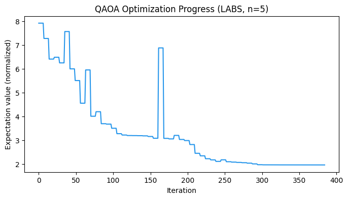
最終サンプリング
最適化されたパラメータでショット数を増やして再度サンプリングします。その後、元のommx.v1.Instanceに対してデコードすることで、返ってくるommx.v1.SampleSetから元のQUBO目的関数の値を直接読み取れます。このQUBO定式化では、補助変数が積を正しく表現しているサンプルではペナルティが発生せず、目的関数値がLABSエネルギーと一致します。一方、という暗黙の関係を破ったサンプルには、ペナルティが加算されます。
def evaluate_with_ommx(
    sample_result, spin_model: BinaryModel, ommx_instance: ommx.v1.Instance
) -> ommx.v1.SampleSet:
    """SPINサンプルをデコードし、BINARYに変換してOMMXインスタンスで評価する。"""
    spin_ss = spin_model.decode_from_sampleresult(sample_result)
    ommx_samples = ommx.v1.Samples({})
    next_id = 0
    for sample, occ in zip(spin_ss.samples, spin_ss.num_occurrences):
        if occ <= 0:
            continue
        # SPIN (+/-1) -> BINARY (0/1): x = (1 - s) / 2
        binary_state = {idx: (1 - val) // 2 for idx, val in sample.items()}
        sample_ids = list(range(next_id, next_id + occ))
        next_id += occ
        ommx_samples.append(
            sample_ids,
            ommx.v1.State({idx: float(val) for idx, val in binary_state.items()}),
        )
    return ommx_instance.evaluate_samples(ommx_samples)


gammas_opt = list(res.x[:p])
betas_opt = list(res.x[p:])
final_shots = 256 if docs_test_mode else 4096

final_result = sampling_executable.sample(
    executor,
    shots=final_shots,
    bindings={"gammas": gammas_opt, "betas": betas_opt},
).result()
qaoa_sample_set = evaluate_with_ommx(final_result, spin_model, instance)

qaoa_summary = qaoa_sample_set.summary
qaoa_best = qaoa_sample_set.best_feasible
qaoa_best_E = int(round(qaoa_best.objective))
ref_E = int(reference_solution.objective)

print(f"Shots:                {len(qaoa_summary)}")
print(f"QAOA best objective:  {qaoa_best_E}")
print(f"Reference E*:         {ref_E}")
Shots: 4096
QAOA best objective: 2
Reference E*: 2
目的関数値の分布
QAOAは一つの解ではなくビット列の分布を返します。下のヒストグラムは、最適化済みパラメータで取得した各ショットのQUBO目的関数の値です。赤の点線は最適値を示します。その線上、またはすぐ右側にあるサンプルは、の値がLABS和を最小化し、の値が積を正しく符号化しています。線から大きく右に離れたサンプルは、の不整合に対するペナルティが加算されています。
objectives = qaoa_summary["objective"].to_numpy()

plt.figure(figsize=(8, 4))
plt.hist(objectives, bins=40, color="#2696EB", edgecolor="white")
plt.axvline(
    ref_E,
    color="red",
    linestyle="--",
    label=f"Reference $E^\\star$ = {ref_E}",
)
plt.xlabel("Objective value (QUBO energy)")
plt.ylabel("Frequency")
plt.title(f"QAOA Output Distribution (p={p}, shots={final_shots})")
plt.legend()
plt.show()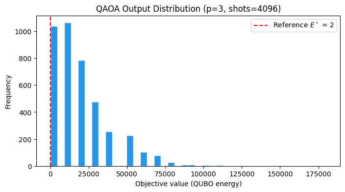
古典ベースライン: OMMXアダプタ経由のSCIP
SCIPは分枝限定法ベースのMILP/QUBOソルバーで、厳密解を求めることができます。同じommx.v1.Instanceをommx_pyscipopt_adapter.OMMXPySCIPOptAdapter.solveに渡すと、PySCIPOpt経由で問題がSCIPに渡され、元のインスタンスに対して評価されたommx.v1.Solutionが返ります。そのため、.objectiveはQAOA側と直接比較できます。
t0 = time.perf_counter()
scip_solution = ommx_pyscipopt_adapter.OMMXPySCIPOptAdapter.solve(instance)
scip_solve_time = time.perf_counter() - t0

scip_E = int(round(scip_solution.objective))
print(f"SCIP E(s):    {scip_E}")
print(f"SCIP feasible: {scip_solution.feasible}")
print(f"Wall time:    {scip_solve_time:.3f} s")
SCIP E(s): 2
SCIP feasible: True
Wall time:    0.095 s
結果の比較
SCIPは最適解を決定論的に返します。一方、QAOAはビット列の分布を返します。そこでQAOA側はベストショット(全サンプル中で最も低い目的関数値を達成したビット列)と、参照最適値に対するヒット率(その値を達成したショットの割合)を見てみます。
# ヒット率: 参照最適値を達成したショットの割合
hit_rate = float((qaoa_summary["objective"].round().astype(int) == ref_E).mean())

print(f"{'Solver':<22} {'E(s)':>8} {'Time (s)':>12}")
print("-" * 46)
print(f"{'Reference (bundled)':<22} {ref_E:>8} {'-':>12}")
print(f"{'SCIP (classical)':<22} {scip_E:>8} {scip_solve_time:>12.3f}")
print(f"{'QAOA (best shot)':<22} {qaoa_best_E:>8} {qaoa_optimize_time:>12.2f}")
print()
print(f"QAOA hit rate on E* = {ref_E}: {hit_rate:.1%}  ({final_shots} shots)")
Solver E(s) Time (s)
----------------------------------------------
Reference (bundled) 2 -
SCIP (classical) 2 0.095
QAOA (best shot) 2 4.40
QAOA hit rate on E* = 2: 4.6% (4096 shots)
このベンチマークから読み取れることは大きく2点あります。
最適値の到達: SCIPとQAOAベストショットのどちらも参照最適値に到達しており、QAOAはかつという軽い設定でも最適系列を見つけられることが分かります。
集中度: QAOAの価値はサンプリング確率を低エネルギーのビット列に集中させる点にあります。上記のヒット率とヒストグラム左端の集中が、その性質を定量化したものです。
なお、経過時間の値はあくまでも参考に留まります。SCIPの計測値はCPU上でのソルバーの実行時間であるのに対し、QAOA側の計測値は状態ベクトルシミュレータ上での古典・量子最適化ループ全体を含み、いずれも実行環境に依存します。このため、実際はより公正な評価方法が必要です。いずれにせよ、OMMX Quantum BenchmarksのようなデータセットとQamomileを組み合わせることで、量子アルゴリズムと古典ソルバーを様々な指標のもとで容易に比較することができます。
まとめ
本チュートリアルでは次のことを行いました。
OMMX Quantum BenchmarksデータセットからLABSインスタンスをそのまま
ommx.v1.Instanceとして読み込みました。Instance.to_qubo()でQUBOを取り出してBinaryModelにラップし、スピン領域に切り替えた上で、@qkernelを使った自作のQAOA ansatzをQiskitTranspiler+AerSimulatorを通じて実行しました。QAOAの出力(ベストショット、ヒット率、サンプリング分布)を、同じインスタンスに対する
ommx_pyscipopt_adapter.OMMXPySCIPOptAdapter.solveの結果、およびベンチマークに同梱された参照最適値と比較しました。
同じパターンは他のQOBLIBデータセット(Marketsplit、IndependentSet、Networkなど)にも適用できます。対応するデータセットクラスでロードし、Instance.to_qubo()でQUBOを取り出して、同じBinaryModel + QAOA ansatz + transpileのループを再利用します。大きなインスタンスがローカルシミュレータの能力を超えた場合は、同じexecutableをQamomileの他のバックエンド(QuriPartsTranspiler、CudaqTranspilerなど)や実機に切り替えられます。