タグ: integration optimization variational
このページでは、具体的な最適化問題を通して、QamomileのQURI Parts量子SDK連携を紹介します。
このチュートリアルでは、小さなMaxCutインスタンスに対するQAOA最適化を例に、Qamomileの量子カーネルをQURI Parts回路へトランスパイルし、サンプリングと期待値評価を行います。
QuriPartsExecutorは、デフォルトで高速なC++製状態ベクトルシミュレータQulacsを使うため、以下の例は追加設定なしでローカルCPU上で実行できます。
# 最新のQamomileをQURI Parts用の追加依存と一緒にpipからインストールします。
# !pip install "qamomile[quri_parts]"
# このチュートリアルで使うライブラリをここにまとめます。
import os
import matplotlib.pyplot as plt
import networkx as nx
import numpy as np
from quri_parts.circuit.noise import ( # type: ignore[import-not-found]
DepolarizingNoise,
NoiseModel,
)
from quri_parts.circuit.utils.circuit_drawer import ( # type: ignore[import-not-found]
draw_circuit,
)
from quri_parts.qulacs.sampler import ( # type: ignore[import-not-found]
create_qulacs_noisesimulator_sampler,
)
from scipy.optimize import minimize
import qamomile.circuit as qmc
import qamomile.observable as qm_o
from qamomile.optimization.binary_model import BinaryModel
from qamomile.quri_parts import QuriPartsExecutor, QuriPartsTranspiler
from qamomile.quri_parts.observable import hamiltonian_to_quri_operatorMaxCut問題
QURI Parts連携の説明に集中するため、MaxCutに対するQAOAチュートリアルと同じ5ノードの小さなグラフを使います。
の最大化は、定数項を除けば、反強磁性Isingハミルトニアンの最小化に対応します。
重みなしMaxCutでは、すべての、なので、これらの係数をそのままBinaryModel.from_isingに渡します。
ここで作るモデルは、QAOAの量子カーネルに渡すquad / linear辞書と、測定結果をスピン値に戻すために使います。
# MaxCutグラフを作り、Ising形式のBinaryModelへ変換します。
G = nx.Graph()
G.add_edges_from([(0, 1), (0, 2), (1, 2), (1, 3), (2, 3), (3, 4)])
num_nodes = G.number_of_nodes()

ising_quad: dict[tuple[int, int], float] = {
    tuple(sorted((i, j))): 1.0 for i, j in G.edges()
}
ising_linear: dict[int, float] = {}
spin_model = BinaryModel.from_ising(linear=ising_linear, quad=ising_quad)
# 問題の構造はグラフから一意に決まります。重みなしMaxCutでは、quad項は辺と
# 1対1に対応し、linear項は存在しません。
assert len(spin_model.quad) == G.number_of_edges()
assert len(spin_model.linear) == 0

pos = nx.spring_layout(G, seed=42)
plt.figure(figsize=(5, 4))
nx.draw(
    G,
    pos,
    with_labels=True,
    node_color="white",
    node_size=700,
    edgecolors="black",
)
plt.title(f"MaxCut graph: {num_nodes} nodes, {G.number_of_edges()} edges")
plt.show()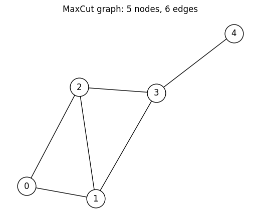
@qkernelによるQAOAアンザッツの構築
QAOAの状態、サンプリング用アンザッツ、期待値計算を、再利用可能な量子カーネルとして書きます。 レシピはMaxCutに対するQAOAチュートリアルと同じです。計算基底の一様な重ね合わせ状態を準備した後、コスト層とミキサー層を回交互に適用します。 サンプリング用の量子カーネルでは最後の状態を計算基底で測定し、期待値計算用の量子カーネルでは同じ状態をHamiltonianに対して評価します。
# QAOAを構成する再利用可能な量子カーネルを定義します。
@qmc.qkernel
def superposition(n: qmc.UInt) -> qmc.Vector[qmc.Qubit]:
q = qmc.qubit_array(n, name="q")
for i in qmc.range(n):
q[i] = qmc.h(q[i])
return q
@qmc.qkernel
def cost_layer(
quad: qmc.Dict[qmc.Tuple[qmc.UInt, qmc.UInt], qmc.Float],
linear: qmc.Dict[qmc.UInt, qmc.Float],
q: qmc.Vector[qmc.Qubit],
gamma: qmc.Float,
) -> qmc.Vector[qmc.Qubit]:
for (i, j), Jij in quad.items():
q[i], q[j] = qmc.rzz(q[i], q[j], angle=Jij * gamma)
for i, hi in linear.items():
q[i] = qmc.rz(q[i], angle=hi * gamma)
return q
@qmc.qkernel
def mixer_layer(
q: qmc.Vector[qmc.Qubit],
beta: qmc.Float,
) -> qmc.Vector[qmc.Qubit]:
n = q.shape[0]
for i in qmc.range(n):
q[i] = qmc.rx(q[i], angle=2.0 * beta)
return q
@qmc.qkernel
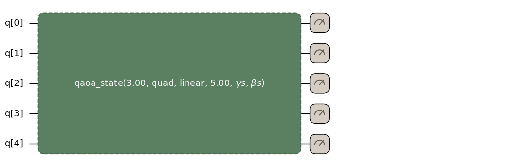
def qaoa_state(
p: qmc.UInt,
quad: qmc.Dict[qmc.Tuple[qmc.UInt, qmc.UInt], qmc.Float],
linear: qmc.Dict[qmc.UInt, qmc.Float],
n: qmc.UInt,
gammas: qmc.Vector[qmc.Float],
betas: qmc.Vector[qmc.Float],
) -> qmc.Vector[qmc.Qubit]:
q = superposition(n)
for layer in qmc.range(p):
q = cost_layer(quad, linear, q, gammas[layer])
q = mixer_layer(q, betas[layer])
return q
@qmc.qkernel
def qaoa_ansatz(
p: qmc.UInt,
quad: qmc.Dict[qmc.Tuple[qmc.UInt, qmc.UInt], qmc.Float],
linear: qmc.Dict[qmc.UInt, qmc.Float],
n: qmc.UInt,
gammas: qmc.Vector[qmc.Float],
betas: qmc.Vector[qmc.Float],
) -> qmc.Vector[qmc.Bit]:
q = qaoa_state(p, quad, linear, n, gammas, betas)
return qmc.measure(q)
@qmc.qkernel
def qaoa_energy(
p: qmc.UInt,
quad: qmc.Dict[qmc.Tuple[qmc.UInt, qmc.UInt], qmc.Float],
linear: qmc.Dict[qmc.UInt, qmc.Float],
n: qmc.UInt,
gammas: qmc.Vector[qmc.Float],
betas: qmc.Vector[qmc.Float],
H: qmc.Observable,
) -> qmc.Float:
q = qaoa_state(p, quad, linear, n, gammas, betas)
return qmc.expval(q, H)qaoa_ansatz.draw(...)でQamomileの回路図を描画できます。
問題の構造を決める引数(p、quad、linear、n)には具体値を渡し、層の形が見えるようにします。
一方、gammas / betasには値を渡さず、後で決めるパラメータとして残します。
p = 3  # QAOAの層数
qaoa_ansatz.draw(
    p=p,
    quad=spin_model.quad,
    linear=spin_model.linear,
    n=num_nodes,
)
QURI Partsへのトランスパイル
QuriPartsTranspilerは、他の量子SDKと同じようにtranspile()で使えます。
問題の構造を決める引数はbindingsで固定し、gammas / betasはランタイムパラメータとして残します。
# seed付きのQURI Parts Executorを作り、アンザッツを1回だけトランスパイルします。
transpiler = QuriPartsTranspiler()

# `seed`を渡すとQulacs samplerが再現可能になります。同じseedと回路で`sample(...)`を2回呼ぶと、まったく同じショットカウントが得られます。
# 非決定的なサンプリングにしたい場合は、この引数を省略する、または`seed=None`を渡してください。
executor = QuriPartsExecutor(seed=42)

executable = transpiler.transpile(
    qaoa_ansatz,
    bindings={
        "p": p,
        "quad": spin_model.quad,
        "linear": spin_model.linear,
        "n": num_nodes,
    },
    parameters=["gammas", "betas"],
)executable.get_first_circuit()で内部のQURI Parts回路を取り出せます。
取り出した回路はQURI PartsのLinearMappedParametricQuantumCircuitであり、個のQAOA角度(gammas[0..p-1]、betas[0..p-1])が名前付きランタイムパラメータとして残っています。
type(...)とパラメータ数で確認し、さらにQURI Partsのdraw_circuitで回路図を描画してみましょう。
# 出力されたQURI Parts回路を確認し、量子ビット数とパラメータ数を検証します。
quri_circuit = executable.get_first_circuit()
assert quri_circuit is not None

# `qubit_count`と`parameter_count`は問題設定から一意に決まります。
# 量子ビット数はグラフのノード数と一致し、ランタイムパラメータ数は層ごとに
# (gamma | beta)の組が1つずつ、合計2pになります。
assert quri_circuit.qubit_count == num_nodes
assert quri_circuit.parameter_count == 2 * p
print(type(quri_circuit).__name__)
print("qubit_count    :", quri_circuit.qubit_count)
print("parameter_count:", quri_circuit.parameter_count)

draw_circuit(quri_circuit, line_length=200)
LinearMappedParametricQuantumCircuit
qubit_count : 5
parameter_count: 6
___ ___ ___ ___ ___ ___ ___ ___ ___ ___
| H | |PPR| |PPR| |PRX| |PPR| |PPR| |PRX| |PPR| |PPR| |PRX|
--|0 |---|5 |---|6 |---|11 |-------------------|16 |---|17 |---|22 |-------------------|27 |---|28 |---|33 |---------------------------------
|___| | | |_ _| |___| | | |_ _| |___| | | |_ _| |___|
___ | | | | ___ ___ ___ | | | | ___ ___ ___ | | | | ___ ___ ___
| H | | | | | |PPR| |PPR| |PRX| | | | | |PPR| |PPR| |PRX| | | | | |PPR| |PPR| |PRX|
--|1 |---| |----| |----|7 |---|8 |---|12 |---| |----| |----|18 |---|19 |---|23 |---| |----| |----|29 |---|30 |---|34 |-----------------
|___| |___| | | | | |_ _| |___| |___| | | | | |_ _| |___| |___| | | | | |_ _| |___|
___ _| |_ | | | | ___ ___ _| |_ | | | | ___ ___ _| |_ | | | | ___ ___
| H | | | | | | | |PPR| |PRX| | | | | | | |PPR| |PRX| | | | | | | |PPR| |PRX|
--|2 |-----------| |---| |----| |----|9 |---|13 |---| |---| |----| |----|20 |---|24 |---| |---| |----| |----|31 |---|35 |---------
|___| |___| |___| | | | | |___| |___| |___| | | | | |___| |___| |___| | | | | |___|
___ _| |_ | | ___ ___ _| |_ | | ___ ___ _| |_ | | ___ ___
| H | | | | | |PPR| |PRX| | | | | |PPR| |PRX| | | | | |PPR| |PRX|
--|3 |---------------------------| |---| |---|10 |---|14 |-----------| |---| |---|21 |---|25 |-----------| |---| |---|32 |---|36 |-
|___| |___| |___| | | |___| |___| |___| | | |___| |___| |___| | | |___|
___ | | ___ | | ___ | | ___
| H | | | |PRX| | | |PRX| | | |PRX|
--|4 |-------------------------------------------| |---|15 |---------------------------| |---|26 |---------------------------| |---|37 |-
|___| |___| |___| |___| |___| |___| |___|
各ランタイムパラメータは、実行時まで未バインドのまま残ります。
そのため、gammas / betasのバインドはQURI Parts側での回路の作り直しではなく、パラメータ値の更新として扱われます。
Ising係数、量子ビット数、層数といった問題構造はトランスパイル時に固定され、ランタイム入力として残るのは変分角度だけです。
QuriPartsExecutorによるQAOAサンプリング
executable.sample(executor, bindings=..., shots=...)はSampleJobを返します。
.result()で得られるSampleResultは、BinaryModel.decode_from_sampleresultでスピン変数のBinarySampleSetへデコードできます。
これにより、追加の変換なしでカット辺を数えられます。
QuriPartsExecutor()は、デフォルトではQulacsの状態ベクトルシミュレータ上で動作します。
rng = np.random.default_rng(42)
init_params = rng.uniform(-np.pi / 2, np.pi / 2, 2 * p)
init_gammas = list(init_params[:p])
init_betas = list(init_params[p:])
docs_test_mode = os.environ.get("QAMOMILE_DOCS_TEST") == "1"
sample_shots = 256 if docs_test_mode else 2000
maxiter = 20 if docs_test_mode else 100

# パラメータ化されたexecutableをサンプリングし、ビット列をIsingエネルギーへデコードします。
sample_result = executable.sample(
    executor,
    bindings={"gammas": init_gammas, "betas": init_betas},
    shots=sample_shots,
).result()

decoded = spin_model.decode_from_sampleresult(sample_result)
print(f"Mean energy at random init: {decoded.energy_mean():+.4f}")
Mean energy at random init: -0.6840
QAOAパラメータの最適化
同じexecutableを異なる(gammas, betas)で繰り返し呼び出すのが、QAOAの最適化ループの基本形です。
transpiler.transpile()を1回呼び、その後はexecutable.sample()を何度も呼び出します。
この例では、サンプリングとデコードの処理をcost_fn()として定義し、SciPyのminimize関数で最適化します。
古典最適化器は(gammas, betas)を更新しながら、サンプリングされたIsingエネルギーの平均を下げていきます。
各反復では、同じexecutableとQuriPartsExecutorを再利用します。
# 1つのexecutableを古典目的関数の中で再利用します。
cost_history: list[float] = []


def cost_fn(params: np.ndarray) -> float:
    result = executable.sample(
        executor,
        bindings={"gammas": list(params[:p]), "betas": list(params[p:])},
        shots=sample_shots,
    ).result()
    energy = spin_model.decode_from_sampleresult(result).energy_mean()
    cost_history.append(energy)
    return energy


# COBYLAでサンプリング平均エネルギーを最適化します。
res = minimize(cost_fn, init_params, method="COBYLA", options={"maxiter": maxiter})

opt_gammas = list(res.x[:p])
opt_betas = list(res.x[p:])
print(f"Optimized mean energy: {res.fun:+.4f}")
print(f"Optimal gammas       : {[round(float(v), 4) for v in opt_gammas]}")
print(f"Optimal betas        : {[round(float(v), 4) for v in opt_betas]}")
Optimized mean energy: -2.8810
Optimal gammas : [0.8678, -0.4364, 1.562]
Optimal betas : [0.4086, -0.8709, 2.9557]
# 最適化の過程における目的関数の変化をプロットします。
plt.figure(figsize=(8, 4))
plt.plot(cost_history, color="#2696EB")
plt.xlabel("Iteration")
plt.ylabel("Cost (mean Ising energy)")
plt.title("QAOA optimization on Qulacs via `QuriPartsExecutor`")
plt.tight_layout()
plt.show()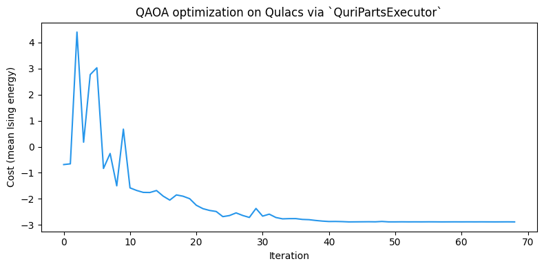
上のQuriPartsExecutorはseed=42で構築しているため、Qulacs samplerは再現可能です。このページを再実行しても、同じ最適化の軌跡と最終エネルギーが得られます。非決定的なサンプリングに戻すには、seed引数を外してください。
この5ノードグラフでは、の基底状態エネルギー付近まで収束するはずです。
ここで得た最適パラメータ(opt_gammas、opt_betas)を、以降の例でも使います。
run()による期待値計算
Qamomileでは、量子回路の出力に対する期待値を量子カーネル内のqmc.expval(...)で記述します。
これをQURI Partsへトランスパイルすると、ExecutableProgram.run(executor, bindings=...)で呼び出せる実行可能オブジェクトになります。
run()はQamomileのパラメータ情報を使ってランタイムパラメータをバインドし、そのうえでQURI Partsのestimatorを呼び出します。
まずをQamomileのHamiltonianとして組み立てます。
その後、期待値計算用の量子カーネルをトランスパイルし、最適化済みQAOAパラメータで評価します。
# MaxCutのIsingコストに対応するQamomileのHamiltonianを組み立てます。
cost_hamiltonian = qm_o.Hamiltonian()
for (i, j), Jij in spin_model.quad.items():
    cost_hamiltonian.add_term(
        (qm_o.PauliOperator(qm_o.Pauli.Z, i), qm_o.PauliOperator(qm_o.Pauli.Z, j)),
        Jij,
    )
for i, hi in spin_model.linear.items():
    cost_hamiltonian.add_term((qm_o.PauliOperator(qm_o.Pauli.Z, i),), hi)

# 期待値計算用の量子カーネルをトランスパイルし、`run()`で評価します。
expval_executable = transpiler.transpile(
    qaoa_energy,
    bindings={
        "p": p,
        "quad": spin_model.quad,
        "linear": spin_model.linear,
        "n": num_nodes,
        "H": cost_hamiltonian,
    },
    parameters=["gammas", "betas"],
)
energy_via_run = expval_executable.run(
    executor,
    bindings={"gammas": opt_gammas, "betas": opt_betas},
).result()

print(f"Executable.run() expectation: {energy_via_run:+.10f}")
print(f"sample mean energy          : {res.fun:+.4f}")
assert np.isfinite(energy_via_run)
Executable.run() expectation: -2.8538574303
sample mean energy : -2.8810
QamomileのAPIだけで扱う場合は、ExecutableProgram.run(...)を使うのがおすすめです。
QURI Parts回路を自分で扱いたい場合にはexecutor.estimate(...)やexecutor.estimate_expectation(...)も使えます。
run()の経路では、Qamomileが名前付きランタイムパラメータをestimator呼び出しの前にバインドするため、QURI Parts側のフラットなパラメータ順をユーザーが管理する必要はありません。
次のセクションでは、より低レベルの経路を開き、QURI Partsが未バインド回路とバインド済み回路をどう扱い分けるかを見ます。
QURI Partsの高度な機能
QURI Partsには、パラメトリックestimatorと非パラメトリックestimatorの両方があります。
Qamomileは通常、この違いをExecutableProgram.run(...)やexecutor.estimate(...)の内側に隠しますが、QURI Parts回路を細かく制御したい場合はestimate_expectation(...)を直接呼び出す方法も便利です。
期待値計算: 未バインド回路とバインド済み回路の違い
QuriPartsExecutor.estimate_expectation(circuit, hamiltonian, param_values)は、QURI Partsで期待値を計算するためのメソッドです。
渡された回路の状態に応じて、QURI Partsの2種類のestimatorを使い分けます。
未バインドのパラメトリック回路:
transpile()が生成した直後の回路は、パラメータをまだ自由変数として保持しています。 QURI Partsのapply_circuitはこれをParametricCircuitQuantumStateで包み、executorはQURI Partsのパラメトリックestimatorを呼び出します。 この場合、評価時にparam_valuesの値でパラメータがバインドされます。バインド済みの回路、もしくは最初からパラメータを持たない回路: 例えば
circuit.bind_parameters([...])を呼んでパラメータを具体的な数値に固定すると、同じapply_circuitはGeneralCircuitQuantumStateを返します。 この場合、executorはQURI Partsの非パラメトリックestimatorを呼び出し、引数のparam_valuesは使われません。
この違いを知っておくと、計算コストを見積もりやすくなります。 同じ回路を異なるパラメータで何度も評価する最適化ループでは、毎回の回路コピーを省けるパラメトリックestimatorが向いています。 逆に、パラメータがすでに具体的な数値に固定されている場合は、パラメトリック回路用の処理が不要な非パラメトリックestimatorのほうが効率的です。
QURI Partsは回路レベルではmeasureを何もしない命令として扱います。
そのため、transpiler.transpile(qaoa_ansatz, ...)が出力するパラメトリック回路は、そのままQAOAの出力状態を準備する回路として使えます。
これをコストハミルトニアンと一緒にestimate_expectationに渡せば、サンプリングノイズを含まないを計算できます。
QAOAの最適化でも、同じ回路を保ったままexecutable.sample()とデコードの組み合わせをexecutor.estimate(circuit, hamiltonian, params=...)に置き換えられます。
2つの経路を直接試すため、前のセクションで作ったHamiltonianをQURI Partsの演算子に変換し、各回路に対してestimate_expectationを呼び出します。
# 直接期待値計算できるよう、observableをQURI Parts演算子へ変換します。
quri_H = hamiltonian_to_quri_operator(cost_hamiltonian)

# transpiler.transpile()直後の、まだバインドされていないパラメトリック回路
unbound_circuit = executable.get_first_circuit()
assert unbound_circuit is not None
print(f"unbound type           : {type(unbound_circuit).__name__}")
print(f"unbound parameter_count: {unbound_circuit.parameter_count}")

# QURI Partsはランタイムパラメータを「回路に登録された順序のフラットなリスト」
# として要求します。登録順は回路を出力したときの初出順で決まるため、QAOAでは
# gammas[0], betas[0], gammas[1], betas[1], ... と層ごとに交互の順になります。
# 「すべてのgammasのあとにすべてのbetas」という順序ではない点に注意してください。
# 順序を推測しなくて済むよう、executableから登録順を読み取り、
# 名前で値を引いてフラットなリストに整えます。
named_values = {f"gammas[{i}]": opt_gammas[i] for i in range(p)}
named_values.update({f"betas[{i}]": opt_betas[i] for i in range(p)})
flat_params = [named_values[name] for name in executable.parameter_names]
# ランタイムパラメータは2p個のQAOA角度のみです。
assert len(executable.parameter_names) == 2 * p
assert len(flat_params) == 2 * p
print(f"circuit parameter order: {executable.parameter_names}")

# QURI Parts標準のバインド処理で、同じ数値を手動でバインドします。
bound_circuit = unbound_circuit.bind_parameters(flat_params)
print(f"bound   type           : {type(bound_circuit).__name__}")

# 経路1: 未バインド回路 → パラメトリックestimator。param_valuesの値が使われます。
energy_unbound = executor.estimate_expectation(
    unbound_circuit, quri_H, flat_params
)

# 経路2: バインド済み回路 → 非パラメトリックestimator。param_valuesは無視されます。
energy_bound = executor.estimate_expectation(bound_circuit, quri_H, [])

print(f"parametric  estimator: {energy_unbound:+.10f}")
print(f"non-param.  estimator: {energy_bound:+.10f}")
assert np.isclose(energy_unbound, energy_bound, atol=1e-10)
assert np.isclose(energy_via_run, energy_unbound, atol=1e-10)
unbound type : LinearMappedParametricQuantumCircuit
unbound parameter_count: 6
circuit parameter order: ['gammas[0]', 'betas[0]', 'gammas[1]', 'betas[1]', 'gammas[2]', 'betas[2]']
bound type : ImmutableBoundParametricQuantumCircuit
parametric estimator: -2.8538574303
non-param. estimator: -2.8538574303
両方の経路は数値精度の範囲で一致します。
同じQAOA状態を、同じIsingコストハミルトニアンに対して評価しているためです。
また、最適化後パラメータでのこのノイズなし期待値は、先ほど出力した標本平均エネルギーともショットノイズの範囲で一致するはずです。
この経路の切り替えはQamomileのexecutor.estimate()インターフェース内部に隠れているので、通常は意識する必要はありません。
estimate_expectationを直接呼び出すのは、QURI Partsの回路を自分で扱う場合に限られます。
executor.estimate(circuit, hamiltonian, params=...)は、既存のQURI Parts回路を渡しつつ、QamomileのHamiltonianオブジェクトをそのまま扱えるメソッドです。
qamomile.observable.Hamiltonianを直接受け取り、内部で自動変換してからestimate_expectationを呼び出します。
# QamomileのHamiltonianをそのまま受け取れるestimatorを使います。
energy_via_estimate = executor.estimate(
    unbound_circuit, cost_hamiltonian, params=flat_params
)
print(f"executor.estimate     : {energy_via_estimate:+.10f}")
assert np.isclose(energy_via_estimate, energy_unbound, atol=1e-10)
executor.estimate : -2.8538574303
他のQURI Parts sampler / estimatorの利用
QuriPartsExecutor()は、初回利用時にデフォルトのQulacs状態ベクトルsamplerとパラメトリックestimatorを遅延生成します。
QURI Partsのsamplerやestimatorを差し替えたい場合は、QuriPartsTranspiler.executor(sampler=..., estimator=...)経由でsamplerやestimatorを渡すか、QuriPartsExecutor(sampler=..., estimator=...)を直接インスタンス化します。
差し替えたexecutorは、上で使ったexecutorの位置にそのまま当てはめられます。
samplerを変えても、量子カーネルをトランスパイルし直す必要はありません。
executableが回路を持ち、executorが実行に使うsamplerやestimatorを持つ、という役割分担になっているためです。
具体例として、QURI PartsのQulacs用NoiseSimulatorを使ったノイズ込みsamplerを構築します。
そして、同じ最適化済みパラメータに対して、ノイズなし版とノイズあり版の標本平均エネルギーを比較します。
すべてのゲートに脱分極ノイズがかかれば、ノイズあり側の平均エネルギーはノイズなしの値からずれるはずです。
これにより、差し替えたsamplerが実際に使われていることを確認できます。
# Qulacsのnoise-simulator samplerを作り、Executorへ渡します。
noise_model = NoiseModel([DepolarizingNoise(error_prob=0.02)])
noisy_sampler = create_qulacs_noisesimulator_sampler(noise_model)
noisy_executor = transpiler.executor(sampler=noisy_sampler)

# 同じexecutableを、ノイズなしsamplerとノイズありsamplerで実行します。
clean_result = executable.sample(
    executor,
    bindings={"gammas": opt_gammas, "betas": opt_betas},
    shots=sample_shots,
).result()
noisy_result = executable.sample(
    noisy_executor,
    bindings={"gammas": opt_gammas, "betas": opt_betas},
    shots=sample_shots,
).result()

# 両方のサンプル集合をデコードし、平均Isingエネルギーを比較します。
clean_energy = spin_model.decode_from_sampleresult(clean_result).energy_mean()
noisy_energy = spin_model.decode_from_sampleresult(noisy_result).energy_mean()
print(f"noiseless sampler mean energy: {clean_energy:+.4f}")
print(f"noisy     sampler mean energy: {noisy_energy:+.4f}")
noiseless sampler mean energy: -2.8810
noisy sampler mean energy: -1.5660
脱分極ノイズはQAOA状態を最大混合状態へ近づけます。
その極限ではすべてのスピン配置が等確率になり、の平均値は0に収束します。
そのため、ノイズあり側の平均エネルギーは、ノイズなしよりも0に近い、つまり高い値になります。
error_probを大きくしたり、ノイズチャネルを追加したりすれば、ノイズあり側のエネルギーはさらに0へ近づきます。
逆にerror_prob=0.0にすれば、ショットノイズの範囲でノイズなしの値に戻ります。
リモートデバイス、密度行列シミュレータ、確率的な状態ベクトルsamplerなど、他のQURI Parts samplerに差し替える場合も同じやり方で動作します。
どの場合でも、量子カーネルの再トランスパイルは不要です。
まとめ
QuriPartsTranspiler().transpile(kernel, bindings=..., parameters=[...])は量子カーネルをQURI PartsのLinearMappedParametricQuantumCircuitに変換し、QURI Partsのdraw_circuitでそのまま確認できます。QuriPartsExecutorは、デフォルトのQulacs状態ベクトルシミュレータ上で、QAOA形式のサンプリングを行うexecutable.sample()、qmc.expval(...)を返す量子カーネル向けのexecutable.run()、回路を直接扱う期待値計算のexecutor.estimate(...)をサポートします。estimate_expectationは、渡された回路にフリーパラメータが残っているかどうかに応じて、QURI Partsのパラメトリックestimatorと非パラメトリックestimatorを切り替えます。通常はexecutor.estimate()を使えば、この切り替えを意識せずに済みます。QURI Partsの
NoiseSimulatorベースのsamplerなど、独自のsamplerやestimatorはtranspiler.executor(...)経由で差し替えられます。量子カーネルをトランスパイルし直す必要はありません。