Pauli Correlation Encoding (PCE)

Tags: algorithm optimization variational

In this tutorial we solve the MaxCut problem with Pauli Correlation Encoding (PCE) using Qamomile’s PCEConverter. PCE maps $N$ spin variables to expectation values of $k$ -body Pauli correlators on a register of $n = \mathcal{O}(N^{1/k})$ qubits. This reduces the qubit count compared with a one-qubit-per-variable QAOA formulation.

We solve a 20-vertex MaxCut instance on 3 qubits with $k = 2$ . The workflow builds the encoding with PCEConverter, estimates each correlator expectation value with a hardware-efficient @qkernel ansatz, optimizes the ansatz with scipy.optimize.minimize, decodes the final expectations with converter.decode, and compares the result with a brute-force baseline.

# Install the latest Qamomile through pip!
# !pip install qamomile

import os

import matplotlib.pyplot as plt
import networkx as nx
import numpy as np
from scipy.optimize import minimize

import qamomile.circuit as qmc
from qamomile.circuit.algorithm.basic import (
    cx_entangling_layer,
    ry_layer,
    rz_layer,
)
from qamomile.optimization.binary_model import BinaryModel, BinarySampleSet
from qamomile.optimization.pce import PCEConverter
from qamomile.qiskit import QiskitTranspiler

Problem Settings¶

What is MaxCut?¶

Given an undirected graph $G = (V, E)$ , the MaxCut problem asks for a partition of the vertices into two sets $S$ and $\bar{S}$ so that the number of edges between the two sets is maximized. We assign each vertex a spin variable $s_i \in \{+1, -1\}$ . The value $s_i = +1$ places vertex $i$ in $S$ , and $s_i = -1$ places it in $\bar{S}$ . The cut value is

\text{MaxCut}(\mathbf{s}) \;=\; \frac{1}{2} \sum_{(i,j) \in E} \bigl(\,1 - s_i s_j\,\bigr).

(1)

Each edge contributes 1 when its endpoints sit on opposite sides ( $s_i s_j = -1$ ) and 0 when they sit on the same side ( $s_i s_j = +1$ ). Maximizing the cut is therefore equivalent to minimizing the Ising energy

E(\mathbf{s}) \;=\; \frac{1}{2} \sum_{(i,j) \in E} s_i s_j \;-\; \frac{|E|}{2}, \qquad E(\mathbf{s}) = -\,\text{MaxCut}(\mathbf{s}),

(2)

This is an Ising model with $h_i = 0$ , $J_{ij} = \tfrac{1}{2}$ on every edge, and a constant offset $-|E|/2$ . PCE works directly with this spin form, so we do not need an extra conversion from binary variables $x \in \{0, 1\}$ .

Create the Graph¶

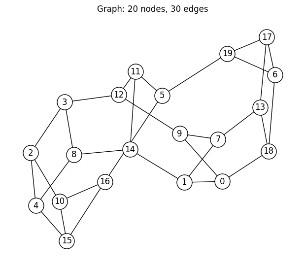
We use a 20-node 3-regular random graph (every vertex has exactly three neighbors, giving $|E| = 3 \cdot 20 / 2 = 30$ edges). MaxCut on a 3-regular graph is a benchmark in the PCE paper. The instance is also small enough for the brute-force baseline to compute the true optimum.

nx.random_regular_graph can produce disconnected graphs, so we increase the seed until the graph is connected. This keeps the example to one partitioning problem instead of several independent components.

seed = 42
while True:
    G = nx.random_regular_graph(3, 20, seed=seed)
    if nx.is_connected(G):
        break
    seed += 1
print(f"Using seed = {seed} (smallest seed >= 42 producing a connected graph)")

num_nodes = G.number_of_nodes()
num_edges = G.number_of_edges()

pos = nx.spring_layout(G, seed=42)
plt.figure(figsize=(6, 5))
nx.draw(
    G,
    pos,
    with_labels=True,
    node_color="white",
    node_size=500,
    edgecolors="black",
)
plt.title(f"Graph: {num_nodes} nodes, {num_edges} edges")
plt.show()

Using seed = 42 (smallest seed >= 42 producing a connected graph)

Algorithm¶

PCE was introduced by Sciorilli et al. Sciorilli et al., 2024 for combinatorial optimization under tight qubit budgets. Standard QAOA uses one qubit per variable. PCE uses $n = \mathcal{O}(N^{1/k})$ qubits for an $N$ -variable problem.

PCE Encoding¶

PCE picks a correlator order $k > 1$ and assigns each spin variable $i \in \{1, \dots, N\}$ to a distinct $k$ -body Pauli correlator $P_i$ . Each $P_i$ is a tensor product of $k$ non-identity Paulis from $\{X, Y, Z\}$ acting on $k$ of the $n$ qubits. The number of distinct such correlators on $n$ qubits is $\binom{n}{k} \cdot 3^k$ , so $n$ is chosen as the smallest integer with

\binom{n}{k} \cdot 3^k \;\ge\; N.

(3)

At $k = 2$ this gives $n = \mathcal{O}(\sqrt{N})$ ; at $k = 3$ it gives $n = \mathcal{O}(N^{1/3})$ . For this $N = 20$ instance, $k = 2$ requires $n = 3$ qubits. This is the smallest integer with $\binom{3}{2} \cdot 9 = 27 \ge 20$ . The mapping from variables to correlators is deterministic: pick any fixed enumeration of $k$ -body Pauli strings on $n$ qubits and assign the first $N$ of them to variables $0, \dots, N-1$ .

Cost Function¶

Given a parameterized ansatz state $|\Psi(\boldsymbol{\theta})\rangle$ , PCE turns the discrete spin objective

C(\mathbf{s}) \;=\; \sum_i h_i \, s_i \,+\, \sum_{i<j} J_{ij} \, s_i s_j

(4)

into a smooth surrogate loss function $\mathcal{L}$ by replacing each spin $s_i$ with the tanh-relaxed correlator expectation $\sigma_i(\boldsymbol{\theta}) = \tanh\bigl(\alpha\, \langle P_i \rangle\bigr)$ , and adding a quartic regularizer that discourages early saturation of the relaxed variables. The tanh map keeps $\sigma_i$ inside the open interval $(-1, +1)$ , where sign rounding can still recover candidate bitstrings:

\mathcal{L}(\boldsymbol{\theta}) \;=\; \underbrace{\sum_i h_i \, \sigma_i \,+\, \sum_{i<j} J_{ij} \, \sigma_i \sigma_j}_{\mathcal{L}_{\text{data}}} \,+\, \mathcal{L}_{\text{reg}}, \qquad \mathcal{L}_{\text{reg}} \;=\; \beta \cdot \nu \cdot \!\left[ \frac{1}{N} \sum_i \sigma_i^2 \right]^{\!2}.

(5)

The data term pulls $\sigma_i$ and $\sigma_j$ toward opposite signs for every connected pair (so $J_{ij} \sigma_i \sigma_j$ is negative); the regularizer counterbalances this pressure by penalizing large relaxed values. This keeps the optimizer in the smooth interior of the domain and reduces early convergence to a suboptimal bitstring.

The loss carries three hyperparameters: $\alpha$ (tanh sharpness), $\beta$ (regularizer strength), and $\nu$ (overall scale). Their values affect optimizer convergence and final solution quality. The concrete values used in this tutorial follow the original paper and are configured in Step 5: Optimize the Variational Parameters.

For MaxCut specifically, the spin model has $h_i = 0$ and $J_{ij} = +\tfrac{1}{2}$ on every edge, so the data term is minimized precisely when adjacent $\sigma_i, \sigma_j$ disagree in sign.

Decoding¶

After convergence, PCE turns each optimized correlator expectation value back into a discrete spin with sign rounding:

s_i \;=\; \operatorname{sgn}\!\bigl\langle P_i \bigr\rangle_{\boldsymbol{\theta}^*} \;\in\; \{+1, -1\},

(6)

i.e. $s_i = +1$ when $\langle P_i \rangle \ge 0$ and $s_i = -1$ otherwise. The binary assignment is recovered as $x_i = (1 - s_i) / 2$ .

Implementation¶

Step 1: Build the `BinaryModel` and `PCEConverter`¶

We build the Ising form derived in Problem Settings with BinaryModel.from_ising: $h_i = 0$ , $J_{ij} = 1/2$ on every edge, and constant $-|E|/2$ . Passing that spin model and correlator order $k = 2$ to PCEConverter lets the converter choose the required qubit count. With this scaling, the spin-model energy equals minus the cut value. A higher cut has a lower energy.

quad = {(i, j): 0.5 for i, j in G.edges()}
ising_model = BinaryModel.from_ising(
    linear={},
    quad=quad,
    constant=-num_edges / 2,
)
converter = PCEConverter(ising_model, correlator_order=2)

spin_model = converter.spin_model
print(f"Number of variables  : {spin_model.num_bits}")
print(f"PCE qubit count      : {converter.num_qubits}")
print(f"Correlator order (k) : {converter.correlator_order}")
print(f"Compression ratio    : {spin_model.num_bits / converter.num_qubits:.1f}x")

assert spin_model.num_bits == 20
assert converter.num_qubits == 3
assert converter.correlator_order == 2

Number of variables  : 20
PCE qubit count      : 3
Correlator order (k) : 2
Compression ratio    : 6.7x

Step 2: Inspect the Per-Variable Pauli Observables¶

get_encoded_pauli_list() returns one Hamiltonian per variable, each containing exactly one $k$ -body Pauli string with coefficient 1. These are the $P_i$ observables from Algorithm. The optimizer will estimate their expectation values with qmc.expval inside the ansatz kernel.

observables = converter.get_encoded_pauli_list()

print(f"Total observables : {len(observables)}")
for i, P_i in enumerate(observables):
    print(f"  P_{i:2d}: {P_i}")

assert len(observables) == spin_model.num_bits
# Each observable is a single k-body Pauli string with coefficient 1.
for P_i in observables:
    coeffs = list(P_i.terms.values())
    assert len(coeffs) == 1 and abs(coeffs[0] - 1.0) < 1e-12

Total observables : 20
  P_ 0: Hamiltonian((X0, X1): 1.0)
  P_ 1: Hamiltonian((X0, Y1): 1.0)
  P_ 2: Hamiltonian((X0, Z1): 1.0)
  P_ 3: Hamiltonian((Y0, X1): 1.0)
  P_ 4: Hamiltonian((Y0, Y1): 1.0)
  P_ 5: Hamiltonian((Y0, Z1): 1.0)
  P_ 6: Hamiltonian((Z0, X1): 1.0)
  P_ 7: Hamiltonian((Z0, Y1): 1.0)
  P_ 8: Hamiltonian((Z0, Z1): 1.0)
  P_ 9: Hamiltonian((X0, X2): 1.0)
  P_10: Hamiltonian((X0, Y2): 1.0)
  P_11: Hamiltonian((X0, Z2): 1.0)
  P_12: Hamiltonian((Y0, X2): 1.0)
  P_13: Hamiltonian((Y0, Y2): 1.0)
  P_14: Hamiltonian((Y0, Z2): 1.0)
  P_15: Hamiltonian((Z0, X2): 1.0)
  P_16: Hamiltonian((Z0, Y2): 1.0)
  P_17: Hamiltonian((Z0, Z2): 1.0)
  P_18: Hamiltonian((X1, X2): 1.0)
  P_19: Hamiltonian((X1, Y2): 1.0)

Step 3: Define the Ansatz¶

PCE leaves the circuit choice open. The original paper uses a hardware-efficient ansatz: alternating layers of single-qubit rotations and two-qubit entangling gates. We use the pre-built ry_layer, rz_layer, and cx_entangling_layer from qamomile.circuit.algorithm.basic and stack them depth times, giving $2 \cdot n \cdot \text{depth}$ variational angles in total. The kernel returns $\langle P \rangle$ , where P is the observable fixed by transpile-time bindings, so we transpile the same kernel once per $P_i$ .

@qmc.qkernel
def pce_ansatz(
    n: qmc.UInt,
    depth: qmc.UInt,
    thetas: qmc.Vector[qmc.Float],
    P: qmc.Observable,
) -> qmc.Float:
    q = qmc.qubit_array(n, name="q")
    for i in qmc.range(n):
        q[i] = qmc.h(q[i])
    for d in qmc.range(depth):
        offset = d * 2 * n
        q = ry_layer(q, thetas, offset)  # type: ignore[arg-type]
        q = rz_layer(q, thetas, offset + n)  # type: ignore[arg-type,operator]
        q = cx_entangling_layer(q)
    return qmc.expval(q, P)

To make the structure concrete, here is the circuit diagram at $n = 3$ qubits and depth = 1 (one layer), with P bound to the first encoded observable. The thetas entries remain runtime parameters.

pce_ansatz.draw(n=3, depth=1, P=observables[0], fold_loops=False)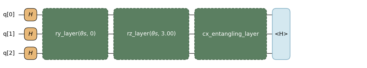

Step 4: Transpile One `ExecutableProgram` per Observable¶

Each $P_i$ must be fixed at transpile time, so we transpile the kernel once per observable and cache the resulting executables. Each transpiler.transpile(...) returns an ExecutableProgram containing the transpiled backend circuit and the metadata needed to rebind runtime parameters. The transpile-time bindings fix the structural inputs (n, depth, P); parameters=["thetas"] leaves the variational angles as runtime parameters that the optimizer can change on every call.

transpiler = QiskitTranspiler()

n = converter.num_qubits
depth = 3
num_thetas = 2 * n * depth

executables = [
    transpiler.transpile(
        pce_ansatz,
        bindings={"n": n, "depth": depth, "P": P_i},
        parameters=["thetas"],
    )
    for P_i in observables
]

print(f"Executables cached : {len(executables)}")
print(f"Variational params : {num_thetas} (= 2 * n * depth)")

assert len(executables) == len(observables)
assert num_thetas == 2 * n * depth

Executables cached : 20
Variational params : 18 (= 2 * n * depth)

Step 5: Optimize the Variational Parameters¶

The classical loop estimates $\langle P_i \rangle$ for every observable at the current thetas, plugs those values into the tanh-relaxed loss from Algorithm (data term + regularizer), and asks scipy.optimize.minimize to update the angles.

We configure the three loss hyperparameters following the original paper:

$\alpha$ (tanh sharpness): set to $\alpha = N^{k/2}$ , where $N$ is the number of graph nodes and $k$ is the correlator order. For our 20-node, $k = 2$ run, $\alpha = 20$ .
$\beta$ (regularizer strength): a fixed value of $1/2$ that the paper has already tuned.
$\nu$ (overall scale): the Edwards–Erdős MaxCut bound, $\nu = |E|/2 + (N - 1)/4$ .

executor = transpiler.executor()
docs_test_mode = os.environ.get("QAMOMILE_DOCS_TEST") == "1"
maxiter = 10 if docs_test_mode else 100

# Hyperparameters from https://doi.org/10.48550/arXiv.2401.09421:
#   alpha = N^(k/2) (N = number of nodes, k = PCE correlator order)
#   beta  = 1/2 (regularizer strength)
#   nu    = |E| / 2 + (N - 1) / 4 (Edwards-Erdős MaxCut bound)
N = spin_model.num_bits
k = converter.correlator_order
alpha = float(N ** (k / 2))
beta = 0.5
nu = num_edges / 2 + (N - 1) / 4
print(f"alpha = {alpha}, beta = {beta}, nu = {nu}")

cost_history: list[float] = []


def measure_expectations(thetas: list[float]) -> list[float]:
    return [
        exe.run(executor, bindings={"thetas": thetas}).result() for exe in executables
    ]


def loss(params: np.ndarray) -> float:
    thetas = list(params)
    expvals = measure_expectations(thetas)
    relaxed = [np.tanh(alpha * e) for e in expvals]

    # Data term: smooth surrogate of the spin objective.
    L_data = 0.0
    for (i, j), J_ij in spin_model.quad.items():
        L_data += J_ij * relaxed[i] * relaxed[j]
    for i, h_i in spin_model.linear.items():
        L_data += h_i * relaxed[i]

    # Regularizer: beta * nu * [(1/N) sum tanh^2(alpha <P_i>)]^2.
    mean_sq = sum(r**2 for r in relaxed) / N
    L_reg = beta * nu * mean_sq**2

    L_total = L_data + L_reg
    cost_history.append(L_total)
    return L_total


rng = np.random.default_rng(42)
initial_params = rng.uniform(-np.pi, np.pi, num_thetas)

res = minimize(loss, initial_params, method="BFGS", options={"maxiter": maxiter})

print(f"Final loss: {res.fun:+.4f}")

alpha = 20.0, beta = 0.5, nu = 19.75

Final loss: -3.4750

plt.figure(figsize=(8, 4))
plt.plot(cost_history, color="#2696EB")
plt.xlabel("Iteration")
plt.ylabel("Loss")
plt.title("PCE Optimization Progress")
plt.show()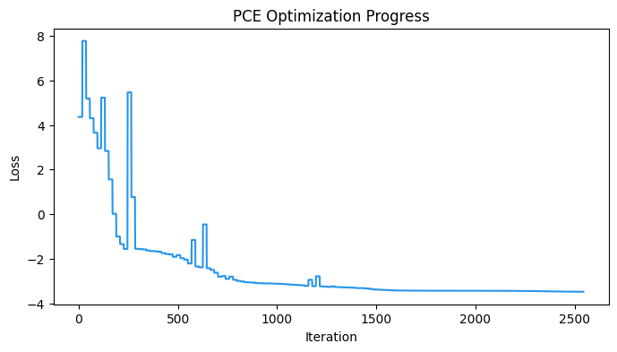

Step 6: Decode the Optimized Expectations¶

PCEConverter.decode(expectations) takes the per-variable expectation values, sign-rounds each one to a spin, and returns a single-sample BinarySampleSet in the same vartype as the input model. Here the vartype is SPIN because ising_model was built with BinaryModel.from_ising. The reported energy follows the convention from Problem Settings: energy = $-\,\text{cut}$ . The decoded energy is the negative of the cut value.

final_expectations = measure_expectations(list(res.x))
sampleset = converter.decode(final_expectations)
# ``PCEConverter`` was built from a ``BinaryModel`` (the ``ising_model``
# above), so ``decode`` returns a ``BinarySampleSet``. The static return
# type is the union ``BinarySampleSet | SampleSet`` because the converter
# class also accepts an OMMX ``Instance``; narrow here so the
# ``.vartype`` / ``.energy`` / ``.samples`` accesses below type-check.
assert isinstance(sampleset, BinarySampleSet)

print("Final per-variable expectations:")
for i, e in enumerate(final_expectations):
    print(f"  <P_{i:2d}> = {e:+.4f}")
print()
print(f"Decoded vartype : {sampleset.vartype}")
print(f"Decoded energy  : {sampleset.energy[0]:+.4f}")

Final per-variable expectations:
  <P_ 0> = -0.0848
  <P_ 1> = +0.0894
  <P_ 2> = +0.3133
  <P_ 3> = -0.0118
  <P_ 4> = -0.0372
  <P_ 5> = -0.2572
  <P_ 6> = -0.0396
  <P_ 7> = -0.0292
  <P_ 8> = +0.0418
  <P_ 9> = +0.2510
  <P_10> = -0.0481
  <P_11> = +0.2302
  <P_12> = -0.2536
  <P_13> = -0.0224
  <P_14> = -0.0883
  <P_15> = +0.0071
  <P_16> = +0.0680
  <P_17> = +0.0666
  <P_18> = +0.3815
  <P_19> = +0.0159

Decoded vartype : SPIN
Decoded energy  : -26.0000

Result¶

Classical Baseline (Brute Force)¶

Enumerating all $2^{20} = 1{,}048{,}576$ spin configurations means checking about one million assignments. That is too many for a simple Python loop, but a single vectorized NumPy pass finishes in a fraction of a second. We label each configuration by an integer whose bit $i$ encodes $s_i = +1$ (bit 0) or $s_i = -1$ (bit 1), then count edges with $s_i \neq s_j$ . This gives us the ground-truth optimum to compare the PCE result against in the next subsection.

assignments = np.arange(2**num_nodes, dtype=np.int64)
cuts = np.zeros(2**num_nodes, dtype=np.int32)
for i, j in G.edges():
    s_i = 1 - 2 * ((assignments >> i) & 1)  # bit 0 → +1, bit 1 → -1
    s_j = 1 - 2 * ((assignments >> j) & 1)
    cuts += (s_i != s_j).astype(np.int32)

best_cut = int(cuts.max())
optimal_assignment_ints = np.flatnonzero(cuts == best_cut)
print(f"Optimal MaxCut value         : {best_cut}")
print(f"Number of optimal partitions : {len(optimal_assignment_ints)}")

# The graph seed is fixed, so the brute-force optimum is deterministic.
assert best_cut == 26

Optimal MaxCut value         : 26
Number of optimal partitions : 12

Decode and Analyze Results¶

Best Cut¶

Convert the decoded spin assignment into a graph partition and compare its cut value with the brute-force optimum from Classical Baseline (Brute Force). As a consistency check, the cut value should equal -1 times the spin energy reported in Step 6: Decode the Optimized Expectations.

sample = sampleset.samples[0]
spins = [sample[i] for i in range(num_nodes)]
pce_cut = sum(1 for i, j in G.edges() if spins[i] != spins[j])

print(f"PCE spin assignment : {spins}")
print(f"PCE cut value       : {pce_cut}")
print(f"Brute-force optimum : {best_cut}")
print(f"Approximation ratio : {pce_cut / best_cut:.3f}")

PCE spin assignment : [-1, 1, 1, -1, -1, -1, -1, -1, 1, 1, -1, 1, -1, -1, -1, 1, 1, 1, 1, 1]
PCE cut value       : 26
Brute-force optimum : 26
Approximation ratio : 1.000

Visualize the Best Solution¶

Color each node by its side of the partition. Nodes with different colors sit on opposite sides of the cut.

color_map = ["#FF6B6B" if spins[i] == 1 else "#4ECDC4" for i in range(num_nodes)]
plt.figure(figsize=(6, 5))
nx.draw(
    G,
    pos,
    with_labels=True,
    node_color=color_map,
    node_size=500,
    edgecolors="black",
)
plt.title(f"PCE partition (cut = {pce_cut} / optimum = {best_cut})")
plt.show()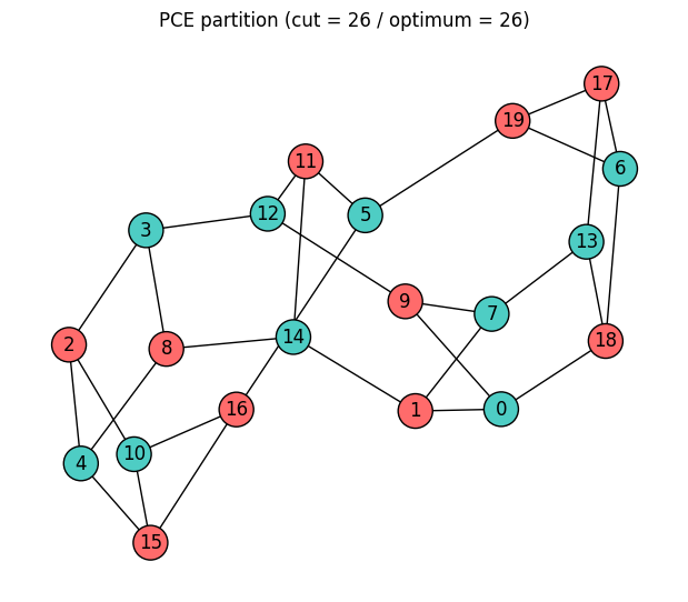

Summary¶

In this tutorial we encoded a 20-node 3-regular MaxCut problem with Pauli Correlation Encoding (PCE) and ran the full Qamomile workflow, from building the correlator encoding through to decoding the optimized expectation values into a spin assignment.

Qubit resource efficiency: PCE represented the 20 spin variables with only 3 qubits through 2-body Pauli correlators, roughly a 7x reduction over the one-qubit-per-variable QAOA encoding.
Surrogate-loss training: the variational loop minimized the tanh-relaxed surrogate rather than an energy directly, and the decoded assignment matched the brute-force optimum.
End-to-end Qamomile path: PCEConverter encoded the given classical variables and exposed the corresponding observables through get_encoded_pauli_list; a hardware-efficient @qkernel ansatz and qmc.expval estimated each correlator; QiskitTranspiler produced the ExecutableProgram objects, the optimizer tuned the parameters, and converter.decode sign-rounded the expectations obtained with those tuned parameters back into the corresponding classical variables.

This PCEConverter workflow applies to any QUBO / Ising combinatorial problem where qubit count is the bottleneck: swap in your own BinaryModel and reuse the encode, transpile, and decode steps shown above.

References¶

Sciorilli, M., Borges, L., Patti, T. L., García-Martín, D., Camilo, G., Anandkumar, A., & Aolita, L. (2024). Towards large-scale quantum optimization solvers with few qubits. 10.48550/ARXIV.2401.09421