Quantum-enhanced Markov chain Monte Carlo

Tags: algorithm sample-based

This tutorial demonstrates how to implement Quantum-enhanced Markov chain Monte Carlo (QeMCMC) Layden et al. (2023) using Qamomile.

# Install the latest Qamomile through pip!
# !pip install qamomile

Background¶

Sampling the Boltzmann Distribution¶

In many physics and engineering problems, drawing samples $\bm{x}$ from a probability distribution $\mu(\bm{x})$ is a central computational task. A classic example is the Boltzmann distribution from statistical mechanics:

\mu(\bm{x}) = \frac{1}{Z} \exp\bigl(-\beta E(\bm{x})\bigr), \quad Z = \sum_{\bm{x}} \exp\bigl(-\beta E(\bm{x})\bigr).

(1)

Here, $E(\bm{x})$ is the energy of state $\bm{x}$ , $\beta = 1/T$ is the inverse temperature, and $Z$ is the normalization constant known as the partition function. Beyond giving the probability distribution of state $\bm{x}$ at thermal equilibrium, sampling that targets the Boltzmann distribution is also widely used as an approach for combinatorial optimization problems.

As a concrete example of an energy function for the Boltzmann distribution, consider the Ising model. The Ising model is a system with a spin variable $x_i \in \{-1, +1\}$ at each site $i$ , whose energy is given by:

E(\bm{x}) = -\sum_{\langle i, j \rangle} J_{ij} \, x_i x_j - \sum_i h_i \, x_i.

(2)

Here, $J_{ij}$ is the interaction between spins and $h_i$ is the external magnetic field at site $i$ . Since the total number of states grows exponentially as $2^n$ , computing the partition function $Z$ exactly becomes intractable for large $n$ . MCMC, introduced below, is therefore used to draw samples directly from $\mu(\bm{x})$ .

First, let us actually visualize the Boltzmann distribution for a small Ising model. We take a 1D ferromagnetic Ising chain ( $J_{i,i+1} = 1$ , $h_i = 0$ ) and plot histograms of the probability aggregated by energy $E(\bm{x})$ for several values of the inverse temperature $\beta$ .

import os
from typing import Any, Callable

import matplotlib.pyplot as plt
import numpy as np

docs_test_mode = os.environ.get("QAMOMILE_DOCS_TEST") == "1"

n_spins = 6
J = 1.0


def ising_energy(state: np.ndarray) -> float:
    """Return the energy of a 1D ferromagnetic Ising chain (no external field)
    for the spin configuration ``state``."""
    return -J * np.sum(state[:-1] * state[1:])


# Enumerate all 2^n states
all_states = np.array(
    [[1 - 2 * ((k >> i) & 1) for i in range(n_spins)] for k in range(2**n_spins)]
)
energies = np.array([ising_energy(s) for s in all_states])
# All 2^n spin configurations on n_spins sites, with energies bounded by
# the ferromagnetic / antiferromagnetic extrema +/- (n - 1) * J.
assert all_states.shape == (2**n_spins, n_spins)
assert energies.shape == (2**n_spins,)
assert energies.min() == -(n_spins - 1) * J
assert energies.max() == (n_spins - 1) * J

# Aggregate the Boltzmann distribution by energy and plot as a histogram
unique_energies = np.unique(energies)
betas = [0.5, 1.0, 2.0]

fig, axes = plt.subplots(1, len(betas), figsize=(12, 3.5), sharey=True)
for ax, beta in zip(axes, betas):
    weights = np.exp(-beta * energies)
    probs = weights / weights.sum()
    e_probs = np.array([probs[energies == e].sum() for e in unique_energies])
    ax.bar(unique_energies, e_probs, width=0.8)
    ax.set_xlabel(r"Energy $E(\mathbf{x})$")
    ax.set_title(rf"$\beta = {beta}$")
axes[0].set_ylabel(r"Probability $\mu(E)$")
fig.suptitle(f"Boltzmann distribution of {n_spins}-spin Ising chain")
plt.tight_layout()
plt.show()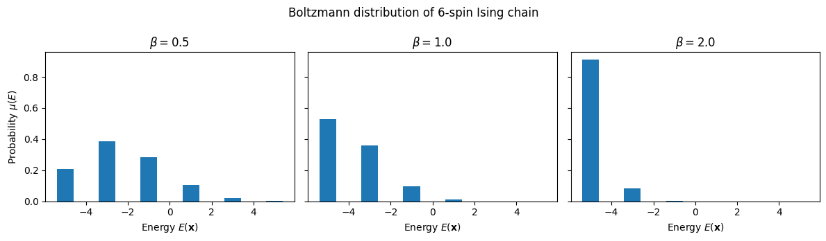

Markov chain Monte Carlo (MCMC)¶

Markov chain Monte Carlo (MCMC) is a general-purpose method for sampling from probability distributions. It achieves sampling from a target distribution $\mu(\bm{x})$ by exploiting a stochastic process called a Markov chain. Here we introduce the Metropolis-Hastings (MH) algorithm Hastings (1970) , a common implementation of MCMC.

The MH algorithm generates a new transition $\bm{x} \rightarrow \bm{y}$ of the Markov chain according to a proposal probability $Q(\bm{y}|\bm{x})$ , and then accepts or rejects this transition according to the acceptance probability

A(\bm{y} | \bm{x}) = \min \left(1, \frac{\mu(\bm{y})}{\mu(\bm{x})} \cdot \frac{Q(\bm{x} | \bm{y})}{Q(\bm{y} | \bm{x})} \right).

(3)

These two steps generate the state at time $t+1$ from the state at time $t$ . After sufficient time, the states of this Markov chain follow the target distribution $\mu(\bm{x})$ . Thus, by running enough transitions, the resulting chain states $\{\bm{x}^{(t)}\}$ can be taken as the desired samples.

Let us verify this in practice. We will sample from the Boltzmann distribution we just prepared using the MH method. Many choices of proposal distribution are possible; here we use the simplest one, which picks a single random spin and flips it.

rng = np.random.default_rng(seed=0)


def local_update(state: np.ndarray) -> np.ndarray:
    """Propose a new spin configuration by flipping a single randomly chosen
    spin in ``state``."""
    n = len(state)
    flip_index = rng.integers(0, n)
    new_state = state.copy()
    new_state[flip_index] = int(-1 * state[flip_index])
    return new_state

Next, we implement the step that stochastically processes the proposed transition according to the acceptance probability. Since this proposal satisfies $Q(\bm{x} \mid \bm{y}) = Q(\bm{y} \mid \bm{x})$ , the ratio of $Q$ cancels out in the acceptance probability. Therefore, when the target distribution is the Boltzmann distribution, the acceptance probability takes the following simple form

A(\bm{y} | \bm{x}) = \min \left(1, \frac{\mu(\bm{y})}{\mu(\bm{x})}\right) = \min \left(1, \exp(-\beta (E(\bm{y}) - E(\bm{x})))\right).

(4)

def metropolis_hastings(
    state: np.ndarray,
    new_state: np.ndarray,
    energy_func: Callable[[np.ndarray], float],
    beta: float,
) -> np.ndarray:
    """Accept or reject ``new_state`` against ``state`` under the
    Metropolis-Hastings rule for the Boltzmann distribution at inverse
    temperature ``beta``."""

    delta_energy = energy_func(new_state) - energy_func(state)

    if delta_energy < 0 or rng.random() < np.exp(
        -beta * delta_energy
    ):  # delta_energy < 0 means the new state has lower energy and is always accepted.
        return new_state
    else:
        return state

Now we have a working MCMC implementation. Let us run it to draw samples.

T = 100 if docs_test_mode else 1000  # Number of MCMC steps
beta = 0.5  # Inverse temperature

sample = np.zeros((T, n_spins))
state = np.ones(n_spins)  # Initial state

for t in range(T):
    new_state = local_update(state)
    state = metropolis_hastings(state, new_state, ising_energy, beta)
    sample[t] = state

Let us confirm that the sampled sequence follows the Boltzmann distribution. Using the samples, we estimate a physical quantity associated with the Boltzmann distribution $\mu(\bm{x})$ . Here we estimate the spin’s average magnetization:

\langle m \rangle = \sum_{\bm{x}} \mu(\bm{x}) m(\bm{x})

(5)

where the magnetization is

m(\bm{x}) = \frac{1}{n} \sum_{i=1}^n x_i.

(6)

Since the average magnetization is the expectation of the magnetization with respect to the Boltzmann distribution, the estimator should become more accurate as the number of samples grows and as the sample distribution gets closer to the Boltzmann distribution. Let us plot the estimator $\bar{m}_t$ obtained from the first $t$ MCMC samples.

def average_magnetization(sample: np.ndarray) -> float:
    """Return the average magnetization estimated from MCMC samples of shape
    ``(T, n_spins)``."""
    magnetization = np.mean(sample, axis=1)
    return np.mean(magnetization)


sample_magnetization = np.array(
    [average_magnetization(sample[:i]) for i in range(1, T + 1)]
)

# Compute the theoretical average magnetization from the Boltzmann distribution
# at the current inverse temperature beta
weights = np.exp(-beta * energies)
probs = weights / weights.sum()
magnetization_per_state = all_states.mean(axis=1)
theoretical_magnetization = np.sum(probs * magnetization_per_state)
# Z2 symmetry: flipping every spin leaves the (h_i = 0) energy invariant
# while negating the magnetization, so the Boltzmann-weighted mean is zero
# exactly — and the per-state contributions cancel exactly in floating
# point because the {+spins, -spins} pairs share the same `probs` value.
assert theoretical_magnetization == 0.0
assert np.isclose(probs.sum(), 1.0)

plt.plot(sample_magnetization, label="MCMC estimate")
plt.axhline(
    theoretical_magnetization,
    color="red",
    linestyle="--",
    label=f"Theoretical ({theoretical_magnetization:.3f})",
)
plt.xlabel("Step")
plt.ylabel("Magnetization")
plt.title("Magnetization vs. Step")
plt.legend()
plt.show()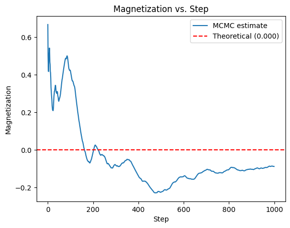

Algorithm¶

The Quantum-enhanced MCMC algorithm is an MCMC that uses sampling from a quantum circuit as its proposal distribution Layden et al. (2023). Starting from the current state $\bm{x}$ , we apply a quantum circuit $U$ and measure in the computational basis to obtain a new state $\bm{y}$ . The resulting proposal distribution $Q(\bm{y}|\bm{x})$ is:

Q(\bm{y}|\bm{x}) = \| \langle \bm{y} | U | \bm{x} \rangle \|^2

(7)

Computing this probability directly is difficult, but when the quantum circuit satisfies $U = U^\top$ , the proposal distribution satisfies $Q(\bm{x} \mid \bm{y}) = Q(\bm{y} \mid \bm{x})$ , so the $Q$ terms cancel out in the acceptance probability, eliminating the need to explicitly compute $Q$ . For example, to sample from the Boltzmann distribution of the Ising model, we can use a trotterized time evolution under a time-independent Hamiltonian:

U(\gamma, t) = \exp(-i H t), \quad \quad H = (1-\gamma) \alpha H_M + \gamma H_C.

(8)

Here, $H_M$ is called the mixer Hamiltonian and generates quantum transitions between states, while $H_C$ is the Ising Hamiltonian. $\gamma \in [0,1]$ is a parameter that controls the relative weights of the two terms. $\alpha$ is a normalization factor used to ensure that the eigenvalues of the mixer and cost Hamiltonians are on the same scale. $(\gamma, t)$ are tunable parameters that determine the efficiency of the MCMC process.

Implementation¶

1. Preparing the Hamiltonians¶

Now let us implement the algorithm. First, we prepare the Ising Hamiltonian $H_C$ for the model we wish to sample and the mixer Hamiltonian $H_M$ for the proposal circuit $U$ .

from qamomile.observable.hamiltonian import Hamiltonian, X, Z

mixer_hamiltonian = Hamiltonian()
for i in range(n_spins):
    mixer_hamiltonian += X(i)

cost_hamiltonian = Hamiltonian()
for i in range(n_spins - 1):
    cost_hamiltonian += -J * Z(i) * Z(i + 1)

2. Building the Quantum Circuit¶

Next, let us implement the quantum circuit. First, we prepare the quantum state $\ket{\bm{x}}$ using computational_basis_state in order to encode the current state $\bm{x}$ as the input state. The proposal transition uses time evolution simulation based on Trotter decomposition. We use trotterized_time_evolution to build the circuit for the Hamiltonians we just prepared.

import qamomile.circuit as qmc
from qamomile.circuit.algorithm import (
    computational_basis_state,
    trotterized_time_evolution,
)


@qmc.qkernel
def qemcmc_circuit(
    n: qmc.UInt,
    input_bits: qmc.Vector[qmc.UInt],
    Hs: qmc.Vector[qmc.Observable],
    order: qmc.UInt,
    time: qmc.Float,
    step: qmc.UInt,
) -> qmc.Vector[qmc.Bit]:
    """QeMCMC proposal circuit: prepare ``|input_bits>`` on ``n`` qubits,
    evolve under ``sum_k Hs[k]`` using a Suzuki-Trotter splitting of given
    ``order`` and ``step`` steps over total time ``time``, then measure all
    qubits."""
    q = qmc.qubit_array(n, name="q")

    # step 1: prepare the initial state
    q = computational_basis_state(q, input_bits)

    # step 2: apply the trotterized evolution under the mixer and cost Hamiltonians
    q = trotterized_time_evolution(q, Hs, order, time, step)

    return qmc.measure(q)

3. Transpiling¶

We transpile the kernel. Running the quantum circuit requires fixed values for the Hamiltonian mixing coefficient $\gamma$ and the simulation time $t$ . Following Christmann et al. (2025) , we set $\gamma=0.45$ , $t=12$ , and $\Delta t = 0.8$ . At transpile time we bind n, order, time, and step, while keeping input_bits as a runtime parameter.

from qamomile.qiskit import QiskitTranspiler

gamma = 0.45  # Mixing coefficient
time = 12.0  # Total evolution time
delta_t = 0.8  # Trotter step size
step = int(time / delta_t)  # Number of Trotter steps
order = 2  # Suzuki-Trotter approximation order
assert step == 15  # 12.0 / 0.8

Hs = [
    (1 - gamma) * mixer_hamiltonian,
    gamma * cost_hamiltonian,
]
assert len(Hs) == 2

transpiler = QiskitTranspiler()

executable = transpiler.transpile(
    qemcmc_circuit,
    bindings={
        "n": n_spins,
        "Hs": Hs,
        "order": order,
        "time": time,
        "step": step,
    },
    parameters=["input_bits"],
)

4. Incorporating the Quantum Circuit into MCMC¶

The quantum circuit simulation is now ready. Finally, let us plug the quantum component into the MCMC. Since the circuit’s input and output are bit strings $\bm{x} \in \{0,1\}^n$ , we also prepare a conversion between bit strings and spin variables $\bm{s} \in \{1, -1\}^n$ .

def spin_binary_convert(x: np.ndarray, *, input_kind: str = "auto") -> np.ndarray:
    """Convert between spin variables {-1, +1} and binary variables {0, 1}.

    ``input_kind`` selects the input convention: ``"spin"`` treats ``x`` as
    {-1, +1} and returns binary, ``"binary"`` treats ``x`` as {0, 1} and
    returns spin. The default ``"auto"`` infers the convention from the
    values, but raises ``ValueError`` for the ambiguous all-ones input.
    """
    x = np.asarray(x, dtype=int)
    values = np.unique(x)

    if input_kind == "spin":
        if not np.all(np.isin(values, [-1, 1])):
            raise ValueError(
                f"input_kind='spin' requires elements in {{-1, 1}}, "
                f"got: {values.tolist()}"
            )
        return (1 - x) // 2
    if input_kind == "binary":
        if not np.all(np.isin(values, [0, 1])):
            raise ValueError(
                f"input_kind='binary' requires elements in {{0, 1}}, "
                f"got: {values.tolist()}"
            )
        return 1 - 2 * x
    if input_kind != "auto":
        raise ValueError(
            f"input_kind must be 'spin', 'binary', or 'auto', got: {input_kind!r}"
        )

    if np.any(values == -1) and np.all(np.isin(values, [-1, 1])):
        return (1 - x) // 2
    if np.any(values == 0) and np.all(np.isin(values, [0, 1])):
        return 1 - 2 * x
    if np.array_equal(values, [1]):
        raise ValueError(
            "Cannot infer spin/binary representation when the input is all ones; "
            "pass input_kind='spin' or input_kind='binary' explicitly."
        )
    raise ValueError(
        f"Elements must be drawn from {{-1, 1}} or {{0, 1}}, got: {values.tolist()}"
    )


def quantum_proposal(state: np.ndarray, executable: Any, executor: Any) -> np.ndarray:
    """Obtain a proposed state from the quantum circuit using the current
    spin state as input."""
    binary_state = spin_binary_convert(state, input_kind="spin").tolist()
    result = executable.sample(
        executor,
        shots=1,
        bindings={"input_bits": binary_state},
    ).result()
    ((proposed_bits, _count),) = result.results
    return spin_binary_convert(np.array(proposed_bits, dtype=int), input_kind="binary")

Example Run¶

Let us run the QeMCMC algorithm we just implemented. We switch to a lower temperature $\beta = 1.0$ where classical local updates mix slowly, so that we can observe the behavior of the quantum proposal distribution under conditions that are harder for the classical baseline. For a fair comparison, we also run a classical MCMC at the same $\beta = 1.0$ alongside the quantum run.

from qiskit_aer import AerSimulator

beta = 1.0  # Switch to a lower temperature where local updates mix slowly
T_quantum = (
    20 if docs_test_mode else 1000
)  # Kept small because quantum-circuit simulation is costly

# Recompute the theoretical average magnetization for the new beta=1.0
weights = np.exp(-beta * energies)
probs = weights / weights.sum()
theoretical_magnetization = np.sum(probs * magnetization_per_state)
# Still zero by Z2 symmetry — beta only reweights pairs, it does not break
# the {+spins, -spins} degeneracy.
assert theoretical_magnetization == 0.0

# Run a classical MCMC at the same beta and step count for a fair comparison
classical_compare_sample = np.zeros((T_quantum, n_spins))
state = np.ones(n_spins)  # Initial state
for t in range(T_quantum):
    new_state = local_update(state)
    state = metropolis_hastings(state, new_state, ising_energy, beta)
    classical_compare_sample[t] = state

# QeMCMC
executor = transpiler.executor(backend=AerSimulator(seed_simulator=7))
quantum_sample = np.zeros((T_quantum, n_spins), dtype=int)
state = np.ones(n_spins, dtype=int)  # Initial state
for t in range(T_quantum):
    proposed_state = quantum_proposal(state, executable, executor)
    state = metropolis_hastings(state, proposed_state, ising_energy, beta)
    quantum_sample[t] = state
# Both chains produced exactly T_quantum samples on n_spins sites with
# spin values restricted to +/- 1.
assert quantum_sample.shape == (T_quantum, n_spins)
assert classical_compare_sample.shape == (T_quantum, n_spins)
assert set(np.unique(quantum_sample).tolist()).issubset({-1, 1})

We compute the estimator of the average magnetization and compare it with the classical MCMC result obtained at the same $\beta = 1.0$ .

quantum_sample_magnetization = np.array(
    [average_magnetization(quantum_sample[:i]) for i in range(1, T_quantum + 1)]
)
classical_compare_magnetization = np.array(
    [average_magnetization(classical_compare_sample[:i]) for i in range(1, T_quantum + 1)]
)

plt.plot(classical_compare_magnetization, label="MCMC estimate")
plt.plot(quantum_sample_magnetization, label="QeMCMC estimate")
plt.axhline(
    theoretical_magnetization,
    color="red",
    linestyle="--",
    label=f"Theoretical ({theoretical_magnetization:.3f})",
)
plt.xlabel("Step")
plt.ylabel("Magnetization")
plt.title("Magnetization vs. Step")
plt.legend()
plt.show()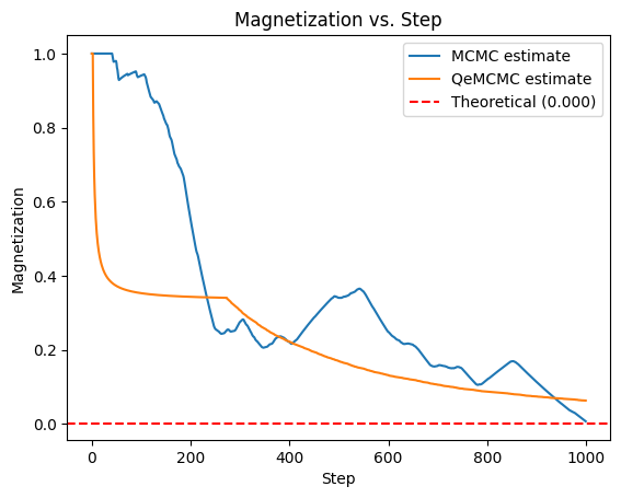

Summary¶

In this tutorial, we began with a review of classical Metropolis-Hastings MCMC and then implemented Quantum-enhanced MCMC (QeMCMC) on top of Qamomile, using the quantum circuit $U(\gamma, t) = \exp(-i t H)$ with $H = (1-\gamma) H_M + \gamma H_C$ as the proposal distribution. Specifically, after preparing the mixer and cost Hamiltonians with qamomile.observable, we built the proposal circuit via Suzuki-Trotter time evolution using trotterized_time_evolution inside an @qkernel. Finally, we plugged the quantum proposal into the existing MH loop through the transpiled executor and compared the convergence of the average magnetization for classical MCMC and QeMCMC on the same Ising chain, confirming that the end-to-end quantum-classical hybrid loop behaves as intended.

References¶

Layden, D., Mazzola, G., Mishmash, R. V., Motta, M., Wocjan, P., Kim, J.-S., & Sheldon, S. (2023). Quantum-enhanced Markov chain Monte Carlo. Nature, 619(7969), 282–287. 10.1038/s41586-023-06095-4
Hastings, W. K. (1970). Monte Carlo sampling methods using Markov chains and their applications. Biometrika, 57(1), 97–109. 10.1093/biomet/57.1.97
Christmann, J., Ivashkov, P., Chiurco, M., & Mazzola, G. (2025). From quantum-enhanced to quantum-inspired Monte Carlo. Physical Review A, 111(4). 10.1103/physreva.111.042615