Grover Adaptive Search for Combinatorial Polynomial Binary Optimization

Tags: algorithm optimization oracle-based

Grover Adaptive Search (GAS) minimizes a polynomial objective over binary variables by repeatedly asking one question of a Grover oracle — which $x$ satisfy $f(x) < y$ ? — and lowering the threshold $y$ whenever a better solution is found Gilliam et al., 2021.

This page solves an unconstrained portfolio selection problem with Qamomile’s GASConverter.

The tutorial is built on the following structure:

Formulate the problem with JijModeling.
Create an instance with concrete data.
Use GASConverter to build the Grover circuit for the current threshold.
Sample it, keep the best candidate, and repeat until a stopping criterion is reached. GAS is a hybrid loop, not a single circuit.

# Install the latest Qamomile through pip!
# !pip install "qamomile[qiskit,visualization]"

import itertools
import os
import random
from typing import Any

import jijmodeling as jm
import numpy as np
from qiskit_aer import AerSimulator

import qamomile.circuit as qmc
from qamomile.circuit.algorithm.gas import (
    apply_function_preparation_qubo,
    diffusion_op,
    grover_algorithm,
)
from qamomile.circuit.visualization import MatplotlibDrawer
from qamomile.optimization.gas import GASConverter
from qamomile.qiskit import QiskitTranspiler

Background¶

Grover search takes an oracle that distinguishes target states by reversing their phase and uses amplitude amplification to raise their measurement probability. That solves a decision problem: a fixed condition says which states qualify, not which one is best.

GAS turns it into minimization by changing this condition. It distinguishes the quantum states corresponding to candidates with $f(x) < y$ by reversing their phase and samples candidates. If a candidate has a lower objective value than the current threshold, the classical layer updates $y$ to that value. This process repeats, with the quantum circuit answering one fixed question at a time and the classical layer updating the threshold.

Problem Settings¶

In this tutorial, we apply GAS to a portfolio selection problem.

Given $n$ assets (stocks, bonds, etc.), we decide for each one whether to buy it — a binary choice. We want to maximize returns while minimizing risk. The tension is:

$\mu$ tells us how profitable each asset is expected to be
$\Sigma$ tells us how assets move together (correlated assets amplify risk)
$q$ controls how much we care about risk vs. return

We need to pick the best subset of assets so that the portfolio earns as much as possible without taking on too much correlated risk.

\min_{x\in \lbrace 0 , 1 \rbrace^n} \big( q x^T \Sigma x - \mu^T x \big)

(1)

@jm.Problem.define("Portfolio Optimization (Unconstrained)")
def portfolio_problem(problem: jm.DecoratedProblem):
    n = problem.Length(description="Number of assets")
    q = problem.Float("q", description="Risk aversion factor")
    mu = problem.Float("mu", shape=(n,), description="Expected returns vector")
    Sigma = problem.Float("Sigma", shape=(n, n), description="Covariance matrix")

    x = problem.BinaryVar("x", shape=(n,), description="1 if asset i is selected")

    problem += (
        q * jm.sum(Sigma[i, j] * x[i] * x[j] for i in n for j in n)
        - jm.sum(mu[i] * x[i] for i in n)
    )


portfolio_problem

The instance below has 9 assets:

Name	Expected Return	Variance
Asset 1	22	12
Asset 2	4	15
Asset 3	19	10
Asset 4	3	18
Asset 5	23	14
Asset 6	2	20
Asset 7	5	11
Asset 8	25	16
Asset 9	3	13

docs_test_mode = os.environ.get("QAMOMILE_DOCS_TEST") == "1"
num_assets = 3 if docs_test_mode else 9
q = 1
mu = np.array([22, 4, 19, 3, 23, 2, 5, 25, 3], dtype=int)
Sigma = np.array([
    [12, -3,  4,  0, -2,  3,  0,  2, -1],
    [-3, 15,  0,  5,  1, -4,  2,  0,  3],
    [ 4,  0, 10, -6,  3,  2, -1,  4,  0],
    [ 0,  5, -6, 18, -4,  0,  3, -2,  5],
    [-2,  1,  3, -4, 14,  2, -3,  0,  2],
    [ 3, -4,  2,  0,  2, 20,  4, -3,  1],
    [ 0,  2, -1,  3, -3,  4, 11,  2, -2],
    [ 2,  0,  4, -2,  0, -3,  2, 16, -4],
    [-1,  3,  0,  5,  2,  1, -2, -4, 13],
], dtype=int)
mu = mu[:num_assets]
Sigma = Sigma[:num_assets, :num_assets]

assert mu.shape == (num_assets,)
assert Sigma.shape == (num_assets, num_assets)
assert np.array_equal(Sigma, Sigma.T), "the covariance matrix must be symmetric"

Evaluating the JijModeling problem with that data yields an OMMX instance.

instance = portfolio_problem.eval({
    "n": num_assets,
    "q": int(q),
    "mu": mu.tolist(),
    "Sigma": Sigma.tolist(),
})

assert len(instance.decision_variables) == num_assets
# The all-zero portfolio buys nothing, so its objective must be exactly 0.
empty_portfolio = instance.evaluate({i: 0 for i in range(num_assets)}).objective
assert np.isclose(empty_portfolio, 0.0, atol=1e-9, rtol=0.0)

Algorithm¶

GAS starts by setting the threshold $y$ to the objective value of a candidate solution and uses Grover search to find candidates with lower objective values. Candidates obtained from the quantum circuit are evaluated classically, and the threshold is updated whenever a better candidate is found. This process repeats until the stopping condition is met. Here $y$ is a threshold on the objective value, not a candidate solution. GAS reverses the phase of the quantum states corresponding to candidates that satisfy $f(x) < y$ , distinguishing them from the other candidates. The Grover ansatz is built from three components:

$A_y$ , the preparation operator. It associates each input with $f(x) - y$ by building the quantum dictionary state $\sum_x \ket{x, f(x) - y}$ . The circuit implementation uses the QFT-based method given in Gilliam et al., 2021. Because the register holds $f(x) - y$ in two’s complement, candidates satisfying the condition can be identified by a Most Significant Bit (MSB) of 1.
$O_y$ , the phase oracle. It reverses the phase of candidates satisfying $f(x) < y$ . The MSB indicates whether the encoded value $f(x) - y$ is negative, so this can be implemented with a single $Z$ gate on that MSB.
$D$ , the diffusion operator, which amplifies the amplitude of the states distinguished by their reversed phase. It is a single multi-controlled- $Z$ sandwiched between $X$ layers.

One iteration applies $O_y$ , then $A_y^\dagger$ , $D$ , $A_y$ . The phase flip on its own leaves every measurement probability unchanged; the reflection $A_y D A_y^\dagger$ is what converts it into amplitude. Measuring the input register returns a candidate, which the classical layer evaluates. It updates $y$ to the candidate’s objective value only if that value is lower than the current threshold.

The remaining question is how many times to apply the Grover operator. GAS answers it by sampling the iteration count from a range that grows slowly whenever a round brings no improvement.

Implementation¶

Qamomile provides the quantum circuits used in GAS through GASConverter. This section introduces its usage and the operations that make up the circuit, then combines them with a classical loop to implement GAS.

GASConverter takes an OMMX instance and converts it into a problem in QUBO/HUBO form. Its transpile() method builds, for a given transpiler, the Grover circuit used by the adaptive search.

converter = GASConverter(instance)
transpiler = QiskitTranspiler()

assert converter.binary_model.num_bits == num_assets

Implementing the Grover circuit¶

GASConverter.transpile() internally builds the sampling qkernel below and feeds it to the transpiler. For visualization we can call Transpiler.to_block and MatplotlibDrawer.draw on that same qkernel.

The output-register width is not a free parameter: it has to hold $f(x) - y$ for every $x$ , or the two’s-complement encoding wraps around and flips the very sign bit the oracle tests. required_output_bits() reports the width transpile() would choose for a given threshold.

output_bits = converter.required_output_bits(y=0)
print(f"Output register width for y=0: {output_bits} qubits")

assert output_bits >= 2

Output register width for y=0: 9 qubits

@qmc.qkernel
def sampling_grover_algorithm(
    n: qmc.UInt,
    m: qmc.UInt,
    y: qmc.Float,
    linear: qmc.Dict[qmc.UInt, qmc.Float],
    quad: qmc.Dict[qmc.Tuple[qmc.UInt, qmc.UInt], qmc.Float],
    iters: qmc.UInt = 1,
) -> tuple[qmc.Vector[qmc.Bit], qmc.Vector[qmc.Bit]]:
    q_output, q_input = grover_algorithm(n, m, y, linear, quad, iters)
    return qmc.measure(q_output), qmc.measure(q_input)


block = transpiler.to_block(
    sampling_grover_algorithm,
    bindings={
        # Number of input qubits = number of binary variables
        "n": converter.binary_model.num_bits,
        # Number of output qubits, as computed by the converter
        "m": output_bits,
        # Oracle threshold: distinguish states for f(x) < y by reversing their phase
        "y": 0,
        "linear": converter.binary_model.linear,
        "quad": converter.binary_model.quad,
        # Number of Grover iterations (can be tuned)
        "iters": 1,
    },
)
block = transpiler.inline(block)

assert len(block.operations) > 0, "the inlined Grover block must not be empty"

MatplotlibDrawer(block).draw(fold_loops=False)

Inspecting the building blocks¶

$A_y$ prepares $\sum_x \ket{x, f(x) - y}$ from QFT phase encodings:

preparation_figure = apply_function_preparation_qubo.draw(
    q_output=output_bits,
    q_input=converter.binary_model.num_bits,
    y=0,
    linear=converter.binary_model.linear,
    quad=converter.binary_model.quad,
    inline=True,
    inline_depth=None,
    fold_loops=False,
)

assert preparation_figure.get_axes(), "the drawn preparation circuit must not be empty"
preparation_figure

and $D$ reflects the input register about the uniform superposition:

diffusion_figure = diffusion_op.draw(
    q_input=converter.binary_model.num_bits,
    inline=True,
    inline_depth=None,
    fold_loops=False,
)

assert diffusion_figure.get_axes(), "the drawn diffusion circuit must not be empty"
diffusion_figure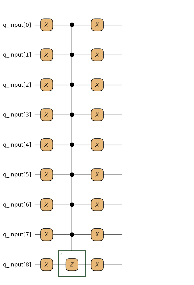

The classical layer¶

Qamomile’s GASConverter provides functionality to construct a Grover circuit for a given threshold and convert measurement results into candidate solutions. However, it does not include the classical logic that controls the overall search: evaluating candidates, updating the threshold, adjusting the number of Grover iterations, and checking the stopping condition. To perform optimization with GAS, you therefore need to implement this logic yourself. The function below is an example of such an implementation.

It implements the classical outer loop of GAS, using converter.transpile() and converter.decode() as its quantum primitives. It starts from a random candidate $x$ with $y = f(x)$ , samples the Grover circuit, and updates the incumbent whenever a sample is better. The search stops after max_no_improvement consecutive rounds without improvement.

converter.transpile(transpiler, y=y, num_iterations=num_iterations) builds the Grover circuit for the current threshold $y$ and the specified number of Grover iterations.
executable.sample(executor, shots=256) runs it on the backend. Even for Grover, multiple shots are needed because NISQ quantum devices are noisy.
converter.decode(result) maps the raw bitstring counts back to decision variable assignments.

def grover_adaptive_search(
    converter: Any,
    transpiler: Any,
    lamb: float,
    max_no_improvement: int = 5,
    shots: int = 256,
    seed: int = 900,
):
    ##########################################################
    #                   Initialization                       #
    ##########################################################

    random.seed(seed)
    n = converter.binary_model.num_bits
    k = 1  # Controls the upper bound of the Grover iteration count sampled per step
    x_int = random.randint(0, 2**n - 1)
    x = [int(b) for b in format(x_int, f"0{n}b")]
    y = converter.instance.evaluate({i: x_i for i, x_i in enumerate(x)}).objective

    current_iter = 0
    no_improvement_count = 0

    print("[GAS] Initialization")
    print(f"[GAS] n={n}, lambda={lamb}")
    print(f"[GAS] Start state: x={x}, y={y}, k={k}")

    executor = transpiler.executor(
        backend=AerSimulator(seed_simulator=seed, max_parallel_threads=None)
    )

    ############################################################
    #                     Main Loop                            #
    ############################################################

    while no_improvement_count < max_no_improvement:
        # Sample t uniformly in {0, ..., ceil(k)-1}; avoid empty range when k == 1
        num_iterations = random.randrange(max(1, int(np.ceil(k))))
        print(
            f"\n[GAS] Iteration {current_iter + 1} | current y={y}, k={k:.6f}, "
            f"Grover iters={num_iterations}"
        )

        ####################################################
        #       Call to the Quantum Grover Circuit         #
        ####################################################

        executable = converter.transpile(
            transpiler, y=y, num_iterations=num_iterations
        )

        # We run the circuit several times since NISQ hardware is noisy
        job = executable.sample(executor, shots=shots)
        result = job.result()
        sample_set = converter.decode(result)

        # Extract x and y from the best sample
        x_vals = sample_set.best_feasible.extract_decision_variables("x")
        candidate_x = [
            int(round(x_vals.get((i,), x_vals.get(i, 0.0)))) for i in range(n)
        ]
        candidate_y = float(sample_set.best_feasible.objective)

        print(f"[GAS] Candidate: x={candidate_x}, y={candidate_y}")

        if candidate_y < y:
            print("[GAS] Improvement found -> accepting candidate and resetting k to 1")
            x = candidate_x
            y = candidate_y
            k = 1
            no_improvement_count = 0
        else:
            old_k = k
            k = lamb * k
            no_improvement_count += 1
            print(
                f"[GAS] No improvement -> keeping current solution and scaling "
                f"k: {old_k:.6f} -> {k:.6f}"
            )

        current_iter += 1

    print(f"\n[GAS] Finished after {current_iter} iterations. Best found: x={x}, y={y}")

    return x, y

Result¶

In this section, we run GAS on the portfolio selection problem and verify the result by comparing the resulting objective value with the optimum obtained by brute-force search.

lamb sets how fast the sampling range for the Grover iteration count grows, and max_no_improvement fixes the stopping criterion.

x, y = grover_adaptive_search(
    converter=converter,
    transpiler=transpiler,
    lamb=1.2,
    max_no_improvement=2 if docs_test_mode else 5,
    shots=16 if docs_test_mode else 256,
    seed=0 if docs_test_mode else 900,
)
selected = [i + 1 for i, xi in enumerate(x) if xi == 1]
print(f"Selected assets: {selected}, objective value: {y}")

assert len(x) == num_assets
assert all(xi in (0, 1) for xi in x)
assert np.isclose(
    y,
    instance.evaluate({i: xi for i, xi in enumerate(x)}).objective,
    atol=1e-9,
    rtol=0.0,
), "the reported objective must match the returned assignment"

[GAS] Initialization
[GAS] n=9, lambda=1.2
[GAS] Start state: x=[0, 1, 1, 1, 0, 1, 0, 0, 1], y=57.0, k=1

[GAS] Iteration 1 | current y=57.0, k=1.000000, Grover iters=0

[GAS] Candidate: x=[1, 0, 1, 1, 1, 0, 0, 0, 0], y=-23.0
[GAS] Improvement found -> accepting candidate and resetting k to 1

[GAS] Iteration 2 | current y=-23.0, k=1.000000, Grover iters=0

[GAS] Candidate: x=[1, 0, 1, 1, 1, 0, 0, 0, 0], y=-23.0
[GAS] No improvement -> keeping current solution and scaling k: 1.000000 -> 1.200000

[GAS] Iteration 3 | current y=-23.0, k=1.200000, Grover iters=0

[GAS] Candidate: x=[1, 0, 1, 1, 1, 0, 0, 0, 0], y=-23.0
[GAS] No improvement -> keeping current solution and scaling k: 1.200000 -> 1.440000

[GAS] Iteration 4 | current y=-23.0, k=1.440000, Grover iters=0

[GAS] Candidate: x=[1, 0, 1, 1, 1, 0, 0, 0, 0], y=-23.0
[GAS] No improvement -> keeping current solution and scaling k: 1.440000 -> 1.728000

[GAS] Iteration 5 | current y=-23.0, k=1.728000, Grover iters=1

[GAS] Candidate: x=[1, 0, 0, 0, 1, 0, 0, 1, 0], y=-28.0
[GAS] Improvement found -> accepting candidate and resetting k to 1

[GAS] Iteration 6 | current y=-28.0, k=1.000000, Grover iters=0

[GAS] Candidate: x=[1, 0, 1, 1, 1, 0, 0, 0, 0], y=-23.0
[GAS] No improvement -> keeping current solution and scaling k: 1.000000 -> 1.200000

[GAS] Iteration 7 | current y=-28.0, k=1.200000, Grover iters=0

[GAS] Candidate: x=[1, 0, 1, 1, 1, 0, 0, 0, 0], y=-23.0
[GAS] No improvement -> keeping current solution and scaling k: 1.200000 -> 1.440000

[GAS] Iteration 8 | current y=-28.0, k=1.440000, Grover iters=1

[GAS] Candidate: x=[1, 0, 0, 0, 1, 0, 0, 1, 0], y=-28.0
[GAS] No improvement -> keeping current solution and scaling k: 1.440000 -> 1.728000

[GAS] Iteration 9 | current y=-28.0, k=1.728000, Grover iters=0

[GAS] Candidate: x=[1, 0, 1, 1, 1, 0, 0, 0, 0], y=-23.0
[GAS] No improvement -> keeping current solution and scaling k: 1.728000 -> 2.073600

[GAS] Iteration 10 | current y=-28.0, k=2.073600, Grover iters=2

[GAS] Candidate: x=[1, 0, 0, 0, 1, 0, 0, 1, 0], y=-28.0
[GAS] No improvement -> keeping current solution and scaling k: 2.073600 -> 2.488320

[GAS] Finished after 10 iterations. Best found: x=[1, 0, 0, 0, 1, 0, 0, 1, 0], y=-28.0
Selected assets: [1, 5, 8], objective value: -28.0

The search stops once the solution has not improved for max_no_improvement rounds, which is a heuristic rule — it does not by itself prove that the returned solution is optimal. With 9 assets, we can enumerate all $2^9 = 512$ assignments, so let’s verify the result against an exact brute-force reference.

brute_force_x, brute_force_y = min(
    (
        (list(bits), instance.evaluate({i: b for i, b in enumerate(bits)}).objective)
        for bits in itertools.product([0, 1], repeat=num_assets)
    ),
    key=lambda candidate: candidate[1],
)

print(f"GAS         : x={x}, objective={y}")
print(f"Brute force : x={brute_force_x}, objective={brute_force_y}")

assert np.isclose(y, brute_force_y, atol=1e-9, rtol=0.0), (
    f"GAS returned objective {y}, but the true optimum is {brute_force_y}"
)
print("\nGAS matched the brute-force optimum.")

GAS         : x=[1, 0, 0, 0, 1, 0, 0, 1, 0], objective=-28.0
Brute force : x=[1, 0, 0, 0, 1, 0, 0, 1, 0], objective=-28.0

GAS matched the brute-force optimum.

Summary¶

In this notebook, we:

Solved an unconstrained portfolio problem with Grover Adaptive Search, where the quantum circuit answers “which $x$ satisfy $f(x) < y$ ?” and a classical loop updates the threshold $y$ when a better candidate is found.
Used GASConverter for the quantum part of GAS: transpile() builds the Grover circuit for the current threshold and number of Grover iterations, and decode() maps bitstring counts back to decision variables through OMMX.
Ran GAS on a portfolio selection problem and verified that the resulting objective value matched the optimum obtained by brute-force search.

References¶

Gilliam, A., Woerner, S., & Gonciulea, C. (2021). Grover Adaptive Search for Constrained Polynomial Binary Optimization. Quantum, 5, 428. 10.22331/q-2021-04-08-428