QSVT Filtering to solve Graph Partitioning

Tags: algorithm optimization oracle-based

This tutorial explains how to use the Quantum Singular Value Transform (QSVT) to find the ground energy of a given Hamiltonian and solve the Graph Partitioning problem.

The ground-energy algorithm of Lin and Tong Lin & Tong, 2020 finds the lowest eigenvalue of a cost Hamiltonian by filtering. For a given threshold parameter $\mu$ , a Linear Combination of Unitaries (LCU) builds a block encoding of $H - \mu I$ . A QSVT approximation of the sign function turns that encoding into a projector onto the eigenspace on one side of $\mu$ . The fraction of shots surviving post-selection tells a classical binary search which way to move $\mu$ .

This notebook runs that whole loop on a graph-partitioning instance and demonstrates how to use the Qamomile library through the QSVTEigenstateFilterConverter: build the block encoding, probe one threshold, then let the binary search locate the ground energy on its own.

# Install the latest Qamomile through pip!
# !pip install "qamomile[qiskit,qsvt,visualization]" networkx

import jijmodeling as jm
import matplotlib.pyplot as plt
import networkx as nx
import numpy as np
from qiskit_aer import AerSimulator

import qamomile.circuit as qmc
from qamomile.circuit.algorithm.qsvt_eigenstate_filter import qsvt_filter_projector
from qamomile.optimization.qsvt_eigenstate_filter import QSVTEigenstateFilterConverter
from qamomile.qiskit import QiskitTranspiler

SEED = 42

Problem Settings¶

Graph partitioning splits the vertices into two equal halves while cutting as few edges as possible. We minimise the number of cut edges subject to an equal-size constraint, which to_hubo absorbs into the objective as a penalty.

See QAOA for Graph Partitioning for more details about the Graph Partitioning problem itself.

problem = jm.Problem("Graph Partitioning")


@problem.update
def _(problem: jm.DecoratedProblem):
    V = problem.Dim()
    E = problem.Natural(ndim=2)  # edge list: [[u1,v1], [u2,v2], ...]
    x = problem.BinaryVar(shape=(V,))

    # Objective: minimize edges cut between partitions
    problem += (
        E.rows().map(lambda e: x[e[0]] * (1 - x[e[1]]) + x[e[1]] * (1 - x[e[0]])).sum()
    )

    # Constraint: equal partition sizes
    problem += problem.Constraint("Equal Partition", x.sum() == V / 2)


problem

num_nodes = 6
# Triangular prism: the triangles {0, 3, 4} and {1, 2, 5} joined by a perfect
# matching (0-5, 1-4, 2-3). Separating the two triangles cuts only the three
# matching edges; every other equal split breaks a triangle and cuts more, so
# the optimal partition is unique.
edge_list = [
    [0, 3],
    [0, 4],
    [0, 5],
    [1, 2],
    [1, 4],
    [1, 5],
    [2, 3],
    [2, 5],
    [3, 4],
]

G = nx.Graph()
G.add_nodes_from(range(num_nodes))
G.add_edges_from(edge_list)
assert G.number_of_nodes() == num_nodes
assert G.number_of_edges() == len(edge_list)

pos = nx.spring_layout(G, seed=1)
plt.figure(figsize=(5, 5))
nx.draw(G, pos, with_labels=True, node_color="white", node_size=700, edgecolors="black")
plt.title(f"Graph: {G.number_of_nodes()} nodes, {G.number_of_edges()} edges")
plt.show()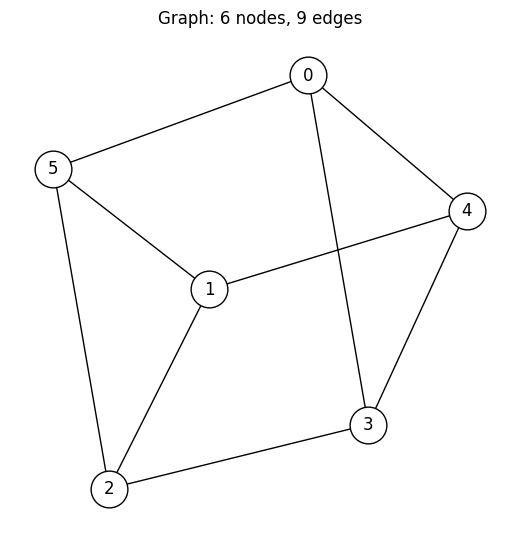

instance_data = {"V": num_nodes, "E": edge_list}
instance = problem.eval(instance_data)

Algorithm¶

Write the Ising cost Hamiltonian as $H$ and pick a threshold $\mu$ . The algorithm works with the shifted operator $H - \mu I$ , whose eigenvalues are $E_i - \mu$ : negative exactly for the eigenstates we want to keep, positive for the rest. Separating the two sides is therefore the job of the sign function.

A block encoding embeds a non-unitary operator as one block of a larger unitary $U$ . LCU builds it by writing $H - \mu I$ as a weighted sum of Pauli strings; the price is a subnormalization $\alpha'$ , so the block actually encoded is the normalized operator $(H - \mu I) / \alpha'$ , whose spectrum lies in $[-1, 1]$ . The block is selected by an ancilla register — the signal register — measuring all zero.

QSVT then replaces the encoded operator by a polynomial of it. Given phases $\Phi$ , it applies the alternation

R(\phi_0),\; U,\; R(\phi_1),\; U^\dagger,\; \dots

(1)

and leaves $p\!\left((H - \mu I)/\alpha'\right)$ in the same block. Choosing $p$ to approximate the sign function,

p\!\left(\frac{H - \mu I}{\alpha'}\right) \approx \operatorname{sign}\!\left(\frac{H - \mu I}{\alpha'}\right),

(2)

makes that block a reflection $R$ : it acts as -1 on the eigenspace below $\mu$ and as +1 on the one above.

A reflection is not yet a projector, but $P_\mu = (I - R)/2$ is, and it is a sum of two unitaries, so a Hadamard test on one extra qubit realises it probabilistically. Starting from the uniform superposition $|\varphi_0\rangle = H^{\otimes n}|0\rangle$ , the fraction of shots with every ancilla measuring zero estimates

P(\mu)=\lVert P_\mu |\varphi_0\rangle \rVert^2 = \frac{\#\{i : E_i < \mu\}}{2^n},

(3)

the fraction of the spectrum below $\mu$ . That single number is the predicate a classical binary search needs: it is bounded away from zero exactly when an eigenstate below $\mu$ carries weight in $|\varphi_0\rangle$ .

The search itself is Algorithm 1 of Lin and Tong Lin & Tong, 2020. Eigenvalues live in $[c-\alpha, c+\alpha)$ , where $\alpha$ is the subnormalization of $H$ alone and $c$ its constant. Compare a threshold $\mu$ to the ground energy $\lambda_0$ : on $[c-\alpha, \lambda_0)$ every eigenvalue is filtered out and $P(\mu)=0$ ; on $[\lambda_0, \lambda_1)$ only the ground eigenspace survives, contributing $\gamma^2 = d/2^n$ for a $d$ -fold degeneracy; above $\lambda_1$ the probability only grows. The search therefore divides $[c-\alpha, c+\alpha)$ into a grid of spacing $h$ and moves according to whether $P(\mu)$ exceeds $\tau = \gamma^2/2$ .

Two inputs make or break it. $\gamma$ is a lower bound on the initial overlap and is not known in advance, so it has to be assumed; and $h$ must be smaller than the (also unknown) spectral gap. Finally, approximation error can make the estimated $P(\mu)$ non-monotonic, so the search evaluates a bracket of two consecutive grid points $(B_k, B_{k+1})$ rather than trusting a single one.

Implementation with Qamomile¶

Qamomile provides the eigenstate-filtering algorithm described above as QSVTEigenstateFilterConverter in qamomile.optimization.qsvt_eigenstate_filter. The converter builds the block encoding of the problem Hamiltonian, synthesizes the filter phases, assembles the probe circuit, and post-selects and decodes the measured samples, so the whole procedure runs directly from the problem instance. Below, we first use it to test one threshold, then open up the building blocks it assembles, and finally drive the binary search with it.

Several internal parameters decide the solution quality, and we explain each of them below, as well as how to choose them.

The constant term of the Ising Hamiltonian is held out of the block encoding. The method’s performance is tied to the subnormalization $\alpha$ , and an identity term makes it grow, while a constant offset shifts every eigenvalue equally without changing which state is best. normalization ( $\alpha$ ) and energy_offset ( $c$ ) together bound the spectrum, and that interval is what a threshold gets chosen against.

converter = QSVTEigenstateFilterConverter(instance)
transpiler = QiskitTranspiler()
# One seeded executor for every circuit on this page, so the printed numbers are
# reproducible from one run to the next.
executor = transpiler.executor(
    backend=AerSimulator(seed_simulator=SEED, max_parallel_threads=1)
)

low = converter.energy_offset - converter.normalization
high = converter.energy_offset + converter.normalization
print(f"alpha={converter.normalization}  offset={converter.energy_offset}")
print(f"every eigenvalue lies in [{low}, {high}]")

# Reference spectrum: the Ising operator is diagonal, so we can read the exact
# energies off directly and check the search against them later.
# !!! This is only a check and the computation takes exponential time in general.
spin = converter.spin_model
energies = np.full(1 << spin.num_bits, float(spin.constant))
for state in range(energies.size):
    for word, coeff in spin.coefficients.items():
        parity = sum((state >> i) & 1 for i in word) & 1
        energies[state] += coeff * (-1.0 if parity else 1.0)

ground_energy = float(energies.min())
degeneracy = int((energies == ground_energy).sum())
print(f"levels={np.unique(energies)}  ground={ground_energy} ({degeneracy}-fold)")

assert low <= energies.min() and energies.max() <= high

alpha=3.0  offset=6.0
every eigenvalue lies in [3.0, 9.0]
levels=[3. 5. 7. 9.]  ground=3.0 (2-fold)

One threshold¶

transpile bakes $\mu$ into the circuit, so each threshold needs its own compilation. The filter keeps the eigenspace below $\mu$ by default, which is what a search for the minimum eigenvalue (ground energy) wants.

degree and delta are paired: delta sets the width of the polynomial’s transition and degree is the degree of the Chebyshev expansion, which must be large enough to represent it.

The resolution is given by

\Delta = \frac{\min_i |E_i-\mu|}{\alpha + |\mu - c|}

(4)

where $E_i$ are the eigenvalues and the other parameters were defined previously. As often, knowing the resolution requires knowing the ground energy in advance; in practice we need to guess or estimate a bound to ensure beating the resolution. The degree roughly scales as $O(1/\Delta)$ .

Below we demonstrate the algorithm for $\mu=4$ . The resolution to beat is then $\Delta = \frac{|4-3|}{3 + |4 - 6|} = 1/5$ , a choice of delta=8 matches the transition to the gap and degree=21 represents it. A bad pairing is not a silent loss of accuracy: it is rejected outright by the $|p| \le 1$ check.

DEGREE, DELTA = 21, 8
SHOTS = 2000
print(f"probe filter: degree={DEGREE}, delta={DELTA} -> {DEGREE + 1} phases")


def probe(mu, shots=SHOTS):
    """Estimate the fraction of the spectrum below `mu`."""
    executable = converter.transpile(
        transpiler,
        mu=mu,
        degree=DEGREE,
        delta=DELTA,
    )
    result = executable.sample(executor, shots=shots).result()
    return converter.success_probability(result)


# Two of the 64 states sit at the ground energy, so the predicate saturates at
# 2 / 64 once mu clears it.
sampled_p4 = probe(4.0)
exact_p4 = float((energies < 4.0).mean())
print(f"p(mu=4.0) = {sampled_p4:.4f}   (exact: {exact_p4:.4f})")

# Six standard deviations of shot noise, plus a small allowance for the blur of
# a finite-degree sign approximation.
shot_noise = 6.0 * np.sqrt(exact_p4 * (1.0 - exact_p4) / SHOTS)
assert abs(sampled_p4 - exact_p4) < shot_noise + 0.01

probe filter: degree=21, delta=8 -> 22 phases

p(mu=4.0) = 0.0310   (exact: 0.0312)

An external library, pyqsp, computes the phase factors corresponding to the polynomial approximation defined by our parameters.

The converter builds the quantum circuit of the projector. The circuit is run and we compute the success probability from the sample counts with the success_probability method. (The exact computation above is only a reference used to check the precision.)

Building blocks¶

transpile composes three circuits, each wrapping the previous one. Drawing them in that order shows how a block encoding becomes a projector.

To keep the pictures readable the phase vector is shortened to four entries (instead of the 22 used above).

DRAW_MU = 4.0

# `_shifted_encoding` is internal: it is not part of the converter's public API,
# but it is the descriptor every circuit below is built from, so the drawings
# match the circuit that actually runs at this threshold.
shifted = converter._shifted_encoding(DRAW_MU)
n_signal = shifted.num_signal_qubits
n_system = shifted.num_system_qubits

# Four phases instead of the 22 the degree-21 filter uses; only the count
# affects the circuit's shape, not the values.
phi_demo = [0.1, 0.2, 0.3, 0.4]

print(f"alpha' = {shifted.normalization}   signal={n_signal}  system={n_system}")

alpha' = 5.0   signal=4  system=6

1. The block encoding $U$ ¶

The Ising Hamiltonian is written as a linear combination of unitaries and realised as $\operatorname{PREPARE}$ , $\operatorname{SELECT}$ , $\operatorname{PREPARE}^\dagger$ . $\operatorname{PREPARE}$ loads the coefficient amplitudes onto the signal register, $\operatorname{SELECT}$ applies the corresponding Pauli- $Z$ term to the system conditioned on the signal, and $\operatorname{PREPARE}^\dagger$ un-computes.

The result is a unitary whose top-left block, the part selected by the signal register measuring all zero, is $(H - \mu I)/\alpha'$ . Nothing outside that block is useful, which is why every shot must be post-selected on it.

@qmc.qkernel
def block_encoding() -> qmc.Vector[qmc.Bit]:
    """Apply the block encoding of (H - mu*I) / alpha' to |0>."""
    signal = qmc.qubit_array(n_signal, "signal")
    system = qmc.qubit_array(n_system, "system")
    signal, system = shifted.unitary(signal, system)
    return qmc.measure(signal)


block_encoding.draw(inline=True, inline_depth=1, fold_loops=False)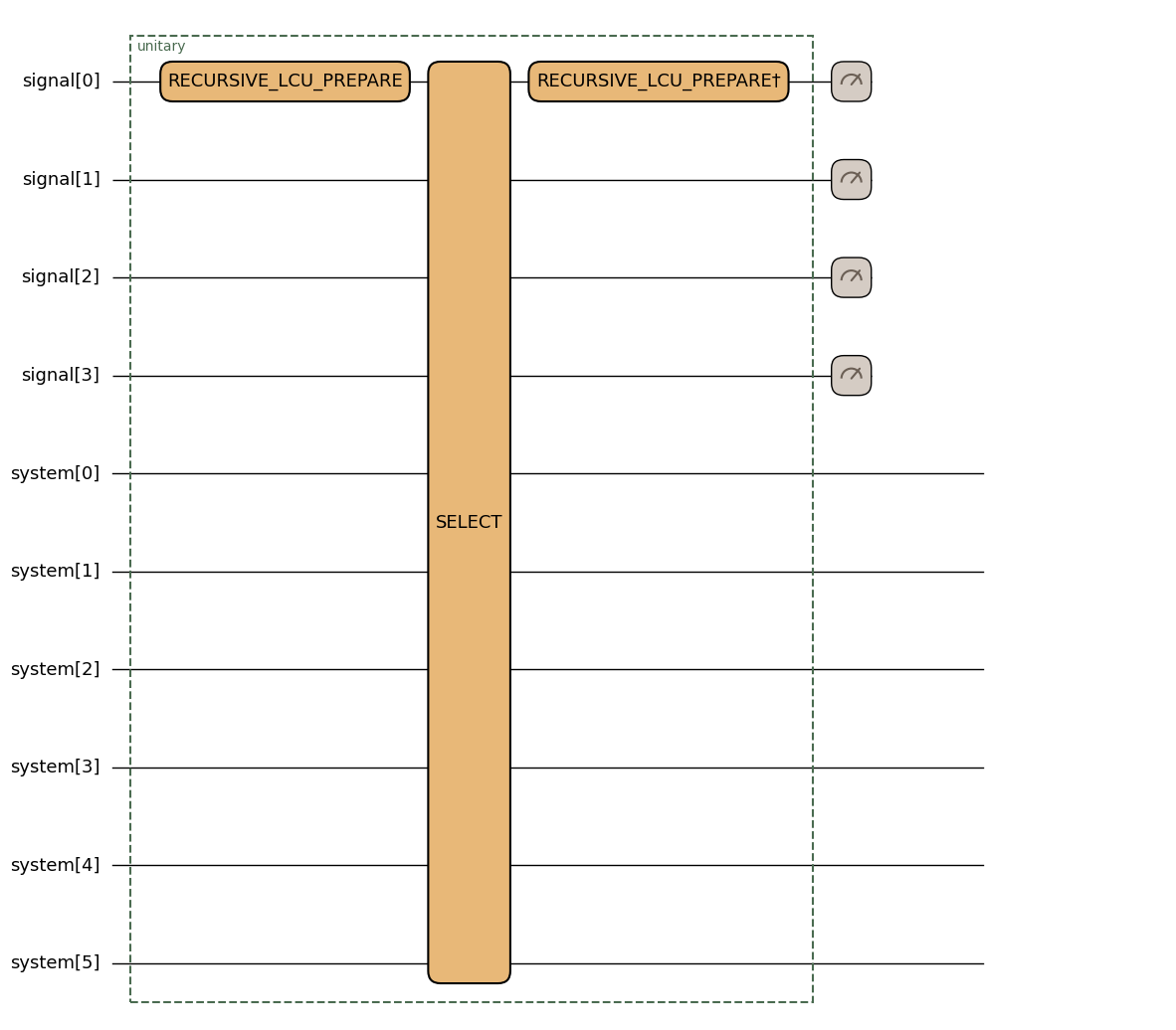

2. The QSVT alternation¶

Given the block encoding, qmc.qsvt applies

R(\phi_0),\; U,\; R(\phi_1),\; U^\dagger,\; R(\phi_2),\; U,\; \dots

(5)

with $U$ the block encoding built above and $R(\phi) = e^{i\phi(2\Pi - I)}$ , where $\Pi$ projects the signal register onto all zero. The primitive owns the whole sequence: it allocates its own rotation auxiliary qubit, alternates $U$ with $U^\dagger$ , and applies the phases.

The effect is to replace the encoded operator by a polynomial of it. With the phases pyqsp produced, that polynomial approximates $\mathrm{sign}$ , so the good block becomes a reflection about the eigenspace on one side of $\mu$ .

@qmc.qkernel
def qsvt_reflector(
    phi: qmc.Vector[qmc.Float],
) -> tuple[qmc.Vector[qmc.Bit], qmc.Vector[qmc.Bit]]:
    """QSVT alternation implementing sign((H - mu*I) / alpha')."""
    signal = qmc.qubit_array(n_signal, "signal")
    system = qmc.qubit_array(n_system, "system")
    signal, system = qmc.qsvt(signal, system, phi, shifted)
    return qmc.measure(signal), qmc.measure(system)


qsvt_reflector.draw(phi=phi_demo, inline=True, inline_depth=0, fold_loops=False)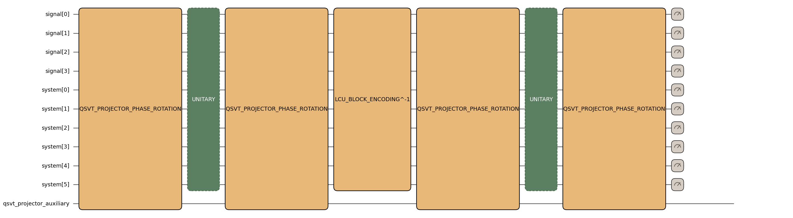

3. The Lin & Tong projector¶

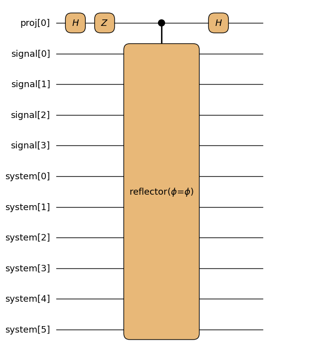
The goal is to turn the reflection into the projection $P_\mu = (I \pm R)/2$ . However, this projector is not unitary, so no circuit can simply apply it.

The trick is that it is a sum of two unitaries, $I$ and $R$ , so a Hadamard test can realise it probabilistically. The test uses one extra ancilla, the probe qubit, which coherently selects between the identity and reflection branches: it is put in superposition, the QSVT reflection is applied under its control, and a second Hadamard interferes the two branches. Measuring the probe qubit as zero heralds the branch where $P_\mu$ was applied; that is why the algorithm has a success probability at all, and why the post-selection is on the probe and the signal register together.

qsvt_filter_projector(shifted).draw(
    proj=1,
    signal=n_signal,
    system=n_system,
    phi=phi_demo,
    inline=True,
    inline_depth=0,
    fold_loops=False,
)

The binary search¶

The predicate is now everything the classical search needs. B(k) is the single bit “the grid point $x_k$ sees the retained eigenspace”, and the loop consumes those bits in consecutive pairs, as described in the Algorithm section.

def binary_search_ground_energy(success_prob, low, high, gamma, h=1.0):
    """Algorithm 1 of Lin & Tong: paired (B_k, B_k+1) probes.

    Grid x_k = low + (k + 0.5) * h: the half-cell offset keeps thresholds
    between candidate energies, since the strict comparison in the predicate
    would read zero on a threshold sitting exactly on an eigenvalue. B_k = 1
    iff the estimated probability exceeds tau = gamma**2 / 2.

    The paired-probe loop narrows to at most four cells; a linear scan over
    those finishes the job, so the returned bracket is one cell wide.
    Returns (x_L, x_U) with x_L <= lambda_0 <= x_U -- closed on the left so a
    ground energy sitting exactly on `low` is still bracketed.
    """
    n_grid = int(round((high - low) / h))
    grid = [low + (k + 0.5) * h for k in range(n_grid)]
    tau = 0.5 * gamma**2
    cache = {}

    def B(k):
        # Boundary sentinels: B_-1 = 0 (nothing below), B_G = 1 (all below).
        if not 0 <= k < n_grid:
            return 0 if k < 0 else 1
        if k not in cache:
            cache[k] = success_prob(grid[k])
        return int(cache[k] > tau)

    L, U = 0, n_grid - 1
    print(f"grid {grid[0]:+.2f}..{grid[-1]:+.2f}  G={n_grid}  h={h}  tau={tau:.4f}")

    while U - L > 3:
        k = (L + U) // 2
        bk, bk1 = B(k), B(k + 1)
        print(f"  k={k}: B({grid[k]:+.2f})={bk}  B({grid[k + 1]:+.2f})={bk1}", end="  ->  ")
        if bk == 1 and bk1 == 1:  # lambda_0 < x_k+1
            U = k + 1
            print(f"(1,1) U<-{U}  [{grid[L]:+.2f}, {grid[U]:+.2f}]")
        elif bk == 0 and bk1 == 0:  # lambda_0 > x_k
            L = k
            print(f"(0,0) L<-{L}  [{grid[L]:+.2f}, {grid[U]:+.2f}]")
        elif bk == 0 and bk1 == 1:  # x_k-1 < lambda_0 < x_k+2
            L, U = max(k - 1, 0), min(k + 2, n_grid - 1)
            print(f"(0,1) -> [{grid[L]:+.2f}, {grid[U]:+.2f}]")
            break
        else:  # x_k < lambda_0 < x_k+1
            L, U = k, k + 1
            print(f"(1,0) -> [{grid[L]:+.2f}, {grid[U]:+.2f}]")
            break

    # Tighten to a single cell: the first grid point whose predicate fires is
    # the smallest threshold that still sees the ground eigenspace. Clamping to
    # the spectrum bound keeps the bracket physical -- no probe is needed below
    # `low`, because no eigenvalue can be there.
    for k in range(L, U + 1):
        if B(k):
            print(f"  refine: first B=1 at k={k} ({grid[k]:+.2f})")
            return max(grid[k] - h, low), grid[k]
    return grid[U], min(grid[U] + h, high)

Result¶

Running the search brackets the ground energy without ever being told where it is. Feeding the resulting threshold back into the filter then prepares the ground state itself, and sampling it recovers the partition.

gamma = np.sqrt(degeneracy / energies.size)
x_lower, x_upper = binary_search_ground_energy(probe, low, high, gamma=gamma, h=1.0)

print(f"\nlambda_0 in [{x_lower:+.2f}, {x_upper:+.2f}]   true lambda_0 = {ground_energy:+.2f}")
assert x_lower <= ground_energy <= x_upper

grid +3.50..+8.50  G=6  h=1.0  tau=0.0156

  k=2: B(+5.50)=1  B(+6.50)=1  ->  (1,1) U<-3  [+3.50, +6.50]

  refine: first B=1 at k=0 (+3.50)

lambda_0 in [+3.00, +3.50]   true lambda_0 = +3.00

# The predicate needed degree 21; extracting the state itself needs a sharper
# filter at the same threshold.
DECODE_DEGREE, DECODE_DELTA = 41, 11
print(
    f"decode filter: degree={DECODE_DEGREE}, delta={DECODE_DELTA} -> {DECODE_DEGREE + 1} phases"
)

executable = converter.transpile(
    transpiler,
    mu=x_upper,
    degree=DECODE_DEGREE,
    delta=DECODE_DELTA,
)
result = executable.sample(executor, shots=20000).result()
sampleset = converter.decode_to_binary_sampleset(result)

kept = sum(sampleset.num_occurrences)
optimal = sum(
    n
    for e, n in zip(sampleset.energy, sampleset.num_occurrences)
    if np.isclose(e, ground_energy)
)
print(f"kept {kept} of {result.shots} shots, {optimal / kept:.1%} at the ground energy")

best = max(zip(sampleset.samples, sampleset.num_occurrences), key=lambda z: z[1])[0]
side = sorted(v for v, bit in best.items() if bit == 1)
cut = sum(1 for u, v in edge_list if best[u] != best[v])
print(f"most sampled partition: {side} | cut={cut}")

assert optimal / kept > 0.85
assert cut == 3 and len(side) == num_nodes // 2

decode filter: degree=41, delta=11 -> 42 phases

kept 531 of 20000 shots, 89.3% at the ground energy
most sampled partition: [1, 2, 5] | cut=3

# Draw the recovered partition on the same layout as the input graph: node
# colour is the side, and the cut edges are the objective being minimised.
cut_edges = [(u, v) for u, v in G.edges() if best[u] != best[v]]
kept_edges = [(u, v) for u, v in G.edges() if best[u] == best[v]]

plt.figure(figsize=(5, 5))
nx.draw_networkx_edges(G, pos, edgelist=kept_edges, edge_color="black", width=1.0)
nx.draw_networkx_edges(
    G, pos, edgelist=cut_edges, edge_color="crimson", width=2.5, style="dashed"
)
nx.draw_networkx_nodes(
    G,
    pos,
    node_color=["#a6cee3" if best[v] == 1 else "#fdbf6f" for v in G.nodes()],
    node_size=700,
    edgecolors="black",
)
nx.draw_networkx_labels(G, pos)
plt.title(f"Recovered partition: {side} vs the rest, cut = {cut} edges")
plt.axis("off")
plt.show()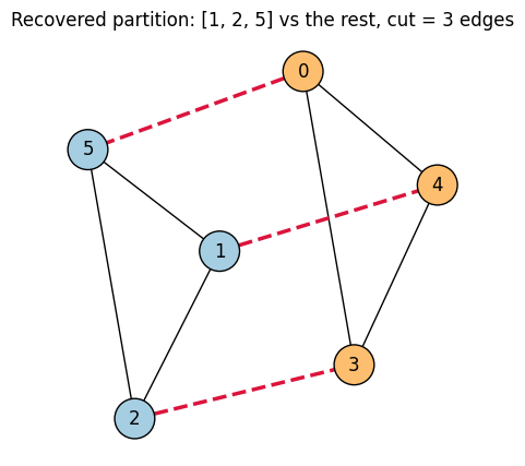

The two triangles $\{0,3,4\}$ and $\{1,2,5\}$ describe the same split, so either side may come out on top from one run to the next; the corresponding objective (minimal cut) is 3.

Summary¶

In this notebook, we:

Solved a graph-partitioning instance end to end with QSVTEigenstateFilterConverter, recovering the unique optimal split of the triangular prism.
Saw why the algorithm is probabilistic: $P_\mu = (I - R)/2$ is not unitary, so a Hadamard test realises it and every shot must be post-selected on the probe and signal registers together.
Saw that every knob traces back to one number, the normalized gap $\Delta = \min_i |E_i - \mu| / \alpha'$ , which is also why holding the Ising constant out of the block encoding matters and why normalization and energy_offset are reported as a pair.

References¶

Lin, L., & Tong, Y. (2020). Near-optimal ground state preparation. 10.48550/ARXIV.2002.12508

QSVT Filtering to solve Graph Partitioning

Problem Settings¶

Algorithm¶

Implementation with Qamomile¶

One threshold¶

Building blocks¶

1. The block encoding UUU¶

2. The QSVT alternation¶

3. The Lin & Tong projector¶

The binary search¶

Result¶

Summary¶

1. The block encoding $U$ ¶